Zero-Based Entry into Financial Risk Control - Loan Default Prediction Challenge
Comprehension of competition questions
The competition question is based on personal credit in financial risk control. Players are required to predict whether the loan applicant is likely to default based on the data information of the loan applicant, so as to determine whether to approve the loan. This is a typical classification problem. Through this competition question, we will guide everyone to understand some business backgrounds in financial risk control, solve practical problems, and help newcomers to the competition practice and improve themselves.
Project address: https://github.com/datawhalechina/team-learning-data-mining/tree/master/FinancialRiskControl
Competition address: https://tianchi.aliyun.com/competition/entrance/531830/introduction
Data form
For the training set data, the characteristics are as follows:
- id The unique letter of credit identifier assigned to the loan list
- loanAmnt loan amount
- term loan period (year)
- interestRate loan interest rate
- installment payment amount
- grade loan grade
- subGrade subgrade of loan grade
- employmentTitle employment title
- employmentLength length of employment (years)
- homeOwnership Home ownership status provided by the borrower at registration
- annualIncome annual income
- verificationStatus verification status
- issueDate The month the loan was issued
- purpose The borrower’s loan purpose category when applying for a loan
- postCode The first 3 digits of the postal code provided by the borrower on the loan application
- regionCode region code
- dti debt to income ratio
- delinquency_2years The number of default events that are more than 30 days overdue in the borrower's credit file in the past 2 years
- ficoRangeLow The lower range of the borrower's fico at the time of loan disbursement
- ficoRangeHigh The upper limit range of the borrower's fico at the time of loan disbursement
- openAcc Number of open credit lines in the borrower's credit file
- pubRec derogates the number of public records
- pubRecBankruptcies Number of public record cleanups
- revolBal total credit revolving balance
- revolUtil Revolving line utilization, or the amount of credit used by a borrower relative to all available revolving credit
- totalAcc The total number of credit lines currently in the borrower's credit file
- initialListStatus The initial list status of the loan
- applicationType indicates whether the loan is an individual application or a joint application with two co-borrowers
- earlyliesCreditLine The month in which the borrower's earliest reported credit line was opened
- title The name of the loan provided by the borrower
- policyCode Publicly available policy_code=1New product Not publicly available policy_code=2
- n series anonymous features Anonymous features n0-n14, processing of some lender behavior counting features
There is also a target column isDefault representing whether there is a default.
Predictive indicators
The competition questions require the use of AUC as the evaluation index.
Specific algorithm
Import related libraries
import pandas as pd
import numpy as np
from sklearn import metrics
import matplotlib.pyplot as plt
from sklearn.metrics import roc_auc_score, roc_curve, mean_squared_error,mean_absolute_error, f1_score
import lightgbm as lgb
import xgboost as xgb
from sklearn.ensemble import RandomForestRegressor as rfr
from sklearn.linear_model import LinearRegression as lr
from sklearn.model_selection import  KFold, StratifiedKFold,GroupKFold, RepeatedKFold
import warnings

warnings.filterwarnings('ignore') #消除warning
Read in data
train_data = pd.read_csv("train.csv")
test_data = pd.read_csv("testA.csv")
print(train_data.shape)
print(test_data.shape)
(800000, 47)
(200000, 47)
data processing
Since the features need to be changed later, I first stacked the training set and the test set together to make it easier to process them together, and then added a column as a distinction.
target = train_data["isDefault"]
train_data["origin"] = "train"
test_data["origin"] = "test"
del train_data["isDefault"]

data = pd.concat([train_data, test_data], axis = 0, ignore_index = True)
data.shape
(1000000, 47)
Then the next step is to process the data. You can first take a look at its general information:
data.info()
<class 'pandas.core.frame.DataFrame'>
RangeIndex: 1000000 entries, 0 to 999999
Data columns (total 47 columns):
 #   Column              Non-Null Count    Dtype
---  ------              --------------    -----
 0   id                  1000000 non-null  int64
 1   loanAmnt            1000000 non-null  float64
 2   term                1000000 non-null  int64
 3   interestRate        1000000 non-null  float64
 4   installment         1000000 non-null  float64
 5   grade               1000000 non-null  object
 6   subGrade            1000000 non-null  object
 7   employmentTitle     999999 non-null   float64
 8   employmentLength    941459 non-null   object
 9   homeOwnership       1000000 non-null  int64
 10  annualIncome        1000000 non-null  float64
 11  verificationStatus  1000000 non-null  int64
 12  issueDate           1000000 non-null  object
 13  purpose             1000000 non-null  int64
 14  postCode            999999 non-null   float64
 15  regionCode          1000000 non-null  int64
 16  dti                 999700 non-null   float64
 17  delinquency_2years  1000000 non-null  float64
 18  ficoRangeLow        1000000 non-null  float64
 19  ficoRangeHigh       1000000 non-null  float64
 20  openAcc             1000000 non-null  float64
 21  pubRec              1000000 non-null  float64
 22  pubRecBankruptcies  999479 non-null   float64
 23  revolBal            1000000 non-null  float64
 24  revolUtil           999342 non-null   float64
 25  totalAcc            1000000 non-null  float64
 26  initialListStatus   1000000 non-null  int64
 27  applicationType     1000000 non-null  int64
 28  earliesCreditLine   1000000 non-null  object
 29  title               999999 non-null   float64
 30  policyCode          1000000 non-null  float64
 31  n0                  949619 non-null   float64
 32  n1                  949619 non-null   float64
 33  n2                  949619 non-null   float64
 34  n3                  949619 non-null   float64
 35  n4                  958367 non-null   float64
 36  n5                  949619 non-null   float64
 37  n6                  949619 non-null   float64
 38  n7                  949619 non-null   float64
 39  n8                  949618 non-null   float64
 40  n9                  949619 non-null   float64
 41  n10                 958367 non-null   float64
 42  n11                 912673 non-null   float64
 43  n12                 949619 non-null   float64
 44  n13                 949619 non-null   float64
 45  n14                 949619 non-null   float64
 46  origin              1000000 non-null  object
dtypes: float64(33), int64(8), object(6)
memory usage: 358.6+ MB
The most important thing is the handling of missing values and outliers, so let’s take a look at which features have the most missing values and outliers:
missing = data.isnull().sum() / len(data)
missing = missing[missing > 0 ]
missing.sort_values(inplace = True)
x = np.arange(len(missing))
fig, ax = plt.subplots()
ax.bar(x,missing)
ax.set_xticks(x)
ax.set_xticklabels(list(missing.index), rotation = 90, fontsize = "small")
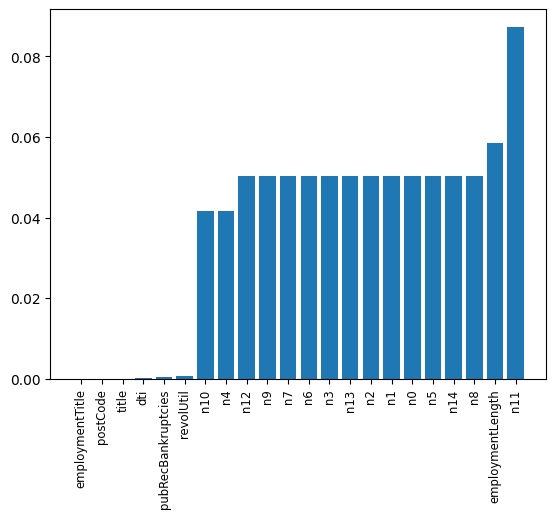
It can be found that there are many outliers in the anonymous features, and there are also many outliers in the employmentLength feature. It will be processed later.
In addition, there are many features that cannot be directly used for training, so they need to be processed, such as grade, subGrade, employmentLength, issueDate, earlyliesCreditLine, which need to be preprocessed.
print(sorted(data['grade'].unique()))
print(sorted(data['subGrade'].unique()))
['A', 'B', 'C', 'D', 'E', 'F', 'G']
['A1', 'A2', 'A3', 'A4', 'A5', 'B1', 'B2', 'B3', 'B4', 'B5', 'C1', 'C2', 'C3', 'C4', 'C5', 'D1', 'D2', 'D3', 'D4', 'D5', 'E1', 'E2', 'E3', 'E4', 'E5', 'F1', 'F2', 'F3', 'F4', 'F5', 'G1', 'G2', 'G3', 'G4', 'G5']
So now let’s deal with the employmentLength feature:
data['employmentLength'].value_counts(dropna=False).sort_index()
1 year        65671
10+ years    328525
2 years       90565
3 years       80163
4 years       59818
5 years       62645
6 years       46582
7 years       44230
8 years       45168
9 years       37866
< 1 year      80226
NaN           58541
Name: employmentLength, dtype: int64
# 对employmentLength该列进行处理
data["employmentLength"].replace(to_replace="10+ years", value = "10 years",
                                      inplace = True)
data["employmentLength"].replace(to_replace="< 1 year", value = "0 years",
                                      inplace = True)
def employmentLength_to_int(s):
    if pd.isnull(s):
        return s # 如果是nan还是nan
    else:
        return np.int8(s.split()[0])  # 按照空格分隔得到第一个字符

data["employmentLength"] = data["employmentLength"].apply(employmentLength_to_int)
The converted effect is:
0.0      80226
1.0      65671
2.0      90565
3.0      80163
4.0      59818
5.0      62645
6.0      46582
7.0      44230
8.0      45168
9.0      37866
10.0    328525
NaN      58541
Name: employmentLength, dtype: int64
The following is the processing of the earlyliesCreditLine time column:
data['earliesCreditLine'].sample(5)
375743    Jun-2003
361340    Jul-1999
716602    Aug-1995
893559    Oct-1982
221525    Nov-2004
Name: earliesCreditLine, dtype: object
For simplicity, let’s just select the year:
data["earliesCreditLine"] = data["earliesCreditLine"].apply(lambda x:int(x[-4:]))
The effect is:
data['earliesCreditLine'].value_counts(dropna=False).sort_index()
1944        2
1945        1
1946        2
1949        1
1950        7
1951        9
1952        7
1953        6
1954        6
1955       10
1956       12
1957       18
1958       27
1959       52
1960       67
1961       67
1962      100
1963      147
1964      215
1965      301
1966      307
1967      470
1968      533
1969      717
1970      743
1971      796
1972     1207
1973     1381
1974     1510
1975     1780
1976     2304
1977     2959
1978     3589
1979     3675
1980     3481
1981     4254
1982     5731
1983     7448
1984     9144
1985    10010
1986    11415
1987    13216
1988    14721
1989    17727
1990    19513
1991    18335
1992    19825
1993    27881
1994    34118
1995    38128
1996    40652
1997    41540
1998    48544
1999    57442
2000    63205
2001    66365
2002    63893
2003    63253
2004    61762
2005    55037
2006    47405
2007    35492
2008    22697
2009    14334
2010    13329
2011    12282
2012     8304
2013     4375
2014     1863
2015      251
Name: earliesCreditLine, dtype: int64
The next step is to process the features of some categories and try to convert them into ont-hot vectors:
cate_features = ["grade",
                "subGrade",
                "employmentTitle",
                "homeOwnership",
                "verificationStatus",
                "purpose",
                "postCode",
                "regionCode",
                "applicationType",
                "initialListStatus",
                "title",
                "policyCode"]
for fea in cate_features:
    print(fea, " 类型数目为:", data[fea].nunique())
grade  类型数目为: 7
subGrade  类型数目为: 35
employmentTitle  类型数目为: 298101
homeOwnership  类型数目为: 6
verificationStatus  类型数目为: 3
purpose  类型数目为: 14
postCode  类型数目为: 935
regionCode  类型数目为: 51
applicationType  类型数目为: 2
initialListStatus  类型数目为: 2
title  类型数目为: 47903
policyCode  类型数目为: 1
It can be seen that some of the features have a relatively small number of categories, so they are suitable for conversion into one-hot vectors, but those with a particularly large number of categories are not suitable. The approach taken by referring to the baseline is to increase the counting and sorting features.
First convert the part to a one-hot vector:
data = pd.get_dummies(data, columns = ['grade', 'subGrade',
                                             'homeOwnership', 'verificationStatus',
                                             'purpose', 'regionCode'],
                     drop_first = True)
# drop_first就是k个类别,我只用k-1个来表示,那个没有表示出来的类别就是全0
For particularly high-dimensional ones:
# 高维类别特征需要进行转换
for f in ['employmentTitle', 'postCode', 'title']:
    data[f+'_cnts'] = data.groupby([f])['id'].transform('count')
    data[f+'_rank'] = data.groupby([f])['id'].rank(ascending=False).astype(int)
    del data[f]

# cnts的意思就是:对f特征的每一个取值进行计数,例如取值A有3个,B有5个,C有7个
# 那么那些f特征取值为A的,在cnt中就是取值为3,B的就是5,C的就是7
# 而rank就是对取值为A的三个排序123,对B的排12345,C的排1234567,各个取值内部排序
# 然后ascending=False就是从后面开始给,最后一个取值为A的给1,倒数第二个给2,倒数第三个给3
The data obtained after processing is:
data.shape
(1000000, 154)
Then it is divided into training data and test data:
train = data[data["origin"] == "train"].reset_index(drop=True)
test = data[data["origin"] == "test"].reset_index(drop=True)
features = [f for f in data.columns if f not in ['id','issueDate','isDefault',"origin"]]  # 这些特征不用参与训练
x_train = train[features]
y_train = target
x_test = test[features]
Select model
I chose xgboost and lightgbm, and then performed model fusion. I will try other combinations when I have time:
lgb_params = {


                'boosting_type': 'gbdt',
                'objective': 'binary',
                'metric': 'auc',
                'min_child_weight': 5,
                'num_leaves': 2 ** 5,
                'lambda_l2': 10,
                'feature_fraction': 0.8,
                'bagging_fraction': 0.8,
                'bagging_freq': 4,
                'learning_rate': 0.1,
                'seed': 2020,
                'nthread': 28,
                'n_jobs':24,
                'verbosity': 1,
                'verbose': -1,
            }
folds = StratifiedKFold(n_splits=5, shuffle=True, random_state=1)
valid_lgb = np.zeros(len(x_train))
predict_lgb = np.zeros(len(x_test))
for fold_, (train_idx,valid_idx) in enumerate(folds.split(x_train, y_train)):
    print("当前第{}折".format(fold_ + 1))
    train_data_now = lgb.Dataset(x_train.iloc[train_idx], y_train[train_idx])
    valid_data_now = lgb.Dataset(x_train.iloc[valid_idx], y_train[valid_idx])
    watchlist = [(train_data_now,"train"), (valid_data_now, "valid_data")]
    num_round = 10000
    lgb_model = lgb.train(lgb_params, train_data_now, num_round,
                        valid_sets=[train_data_now, valid_data_now], verbose_eval=500,
                       early_stopping_rounds = 800)
    valid_lgb[valid_idx] = lgb_model.predict(lgb.Dataset(x_train.iloc[valid_idx]),
                                           ntree_limit = lgb_model.best_ntree_limit)
    predict_lgb += lgb_model.predict(lgb.Dataset(x_test), num_iteration=
                                           lgb_model.best_iteration) / folds.n_splits
This part of the training process has been introduced in my previous integrated learning practical blog, so I also apply that part of the idea.
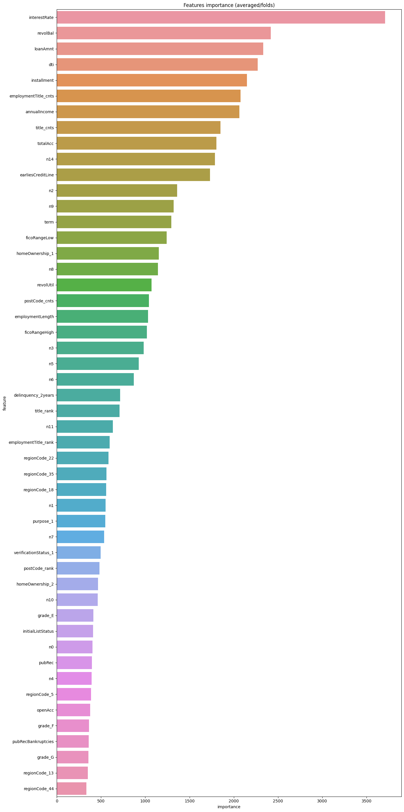
Likewise, you can also look at feature importance:
pd.set_option("display.max_columns", None)  # 设置可以显示的最大行和最大列
pd.set_option('display.max_rows', None)  # 如果超过就显示省略号,none表示不省略
#设置value的显示长度为100,默认为50
pd.set_option('max_colwidth',100)
df = pd.DataFrame(data[features].columns.tolist(), columns=['feature'])
df['importance'] = list(lgb_model.feature_importance())
df = df.sort_values(by = "importance", ascending=False)
plt.figure(figsize = (14,28))
sns.barplot(x = 'importance', y = 'feature', data = df.head(50))
plt.title('Features importance (averaged/folds)')
plt.tight_layout()  # 自动调整适应范围
# xgboost模型

xgb_params = {

    'booster': 'gbtree',
                      'objective': 'binary:logistic',
                      'eval_metric': 'auc',
                      'gamma': 1,
                      'min_child_weight': 1.5,
                      'max_depth': 5,
                      'lambda': 10,
                      'subsample': 0.7,
                      'colsample_bytree': 0.7,
                      'colsample_bylevel': 0.7,
                      'eta': 0.04,
                      'tree_method': 'exact',
                      'seed': 1,
                      'nthread': 36,
                      "verbosity": 1,
                      }
folds = StratifiedKFold(n_splits=5, shuffle=True, random_state=1)
valid_xgb = np.zeros(len(x_train))
predict_xgb = np.zeros(len(x_test))
for fold_, (train_idx,valid_idx) in enumerate(folds.split(x_train, y_train)):
    print("当前第{}折".format(fold_ + 1))
    train_data_now = xgb.DMatrix(x_train.iloc[train_idx], y_train[train_idx])
    valid_data_now = xgb.DMatrix(x_train.iloc[valid_idx], y_train[valid_idx])
    watchlist = [(train_data_now,"train"), (valid_data_now, "valid_data")]
    xgb_model = xgb.train(dtrain = train_data_now, num_boost_round = 3000,
                         evals = watchlist, early_stopping_rounds = 500,
                         verbose_eval = 500, params = xgb_params)
    valid_xgb[valid_idx] =xgb_model.predict(xgb.DMatrix(x_train.iloc[valid_idx]),
                                           ntree_limit = xgb_model.best_ntree_limit)
    predict_xgb += xgb_model.predict(xgb.DMatrix(x_test),ntree_limit
                                     = xgb_model.best_ntree_limit) / folds.n_splits
Let’s take a look at part of the training process:
当前第5折
[0]	train-auc:0.69345	valid_data-auc:0.69341
[500]	train-auc:0.73811	valid_data-auc:0.72788
[1000]	train-auc:0.74875	valid_data-auc:0.73066
[1500]	train-auc:0.75721	valid_data-auc:0.73194
[2000]	train-auc:0.76473	valid_data-auc:0.73266
[2500]	train-auc:0.77152	valid_data-auc:0.73302
[2999]	train-auc:0.77775	valid_data-auc:0.73307
Then I used simple logistic regression for the next model fusion:
# 模型融合
train_stack = np.vstack([valid_lgb, valid_xgb]).transpose()
test_stack = np.vstack([predict_lgb, predict_xgb]).transpose()
folds_stack = RepeatedKFold(n_splits = 5, n_repeats = 2, random_state = 1)
valid_stack = np.zeros(train_stack.shape[0])
predict_lr2 = np.zeros(test_stack.shape[0])

for fold_, (train_idx, valid_idx) in enumerate(folds_stack.split(train_stack, target)):
    print("当前是第{}折".format(fold_+1))
    train_x_now, train_y_now = train_stack[train_idx], target.iloc[train_idx].values
    valid_x_now, valid_y_now = train_stack[valid_idx], target.iloc[valid_idx].values
    lr2 = lr()
    lr2.fit(train_x_now, train_y_now)
    valid_stack[valid_idx] = lr2.predict(valid_x_now)
    predict_lr2 += lr2.predict(test_stack) / 10

print("score:{:<8.8f}".format(roc_auc_score(target, valid_stack)))
score:0.73229269
Predict and save
testA = pd.read_csv("testA.csv")
testA['isDefault'] = predict_lr2
submission_data = testA[['id','isDefault']]
submission_data.to_csv("myresult.csv",index = False)
Now you can submit it!
Complete!