Getting Started with OpenCV (14) Quickly Learn OpenCV 13 Edge Detection

Author: Xiou

1. Overview of edge detection

Edge detection is a basic problem in image processing and computer vision. The purpose of edge detection is to identify points in digital images with obvious brightness changes. Significant changes in image properties often reflect important events and changes in properties, including depth discontinuities, surface orientation discontinuities, material property changes, and scene lighting changes. Edge detection features are an area of ​​research in extraction. Image edge detection greatly reduces the amount of data, eliminates information that can be considered irrelevant, and retains important structural attributes of the image.

There are many methods for edge detection, most of which can be divided into two categories: one based on search and one based on zero crossing. Search-based methods detect boundaries by finding the maximum and minimum values ​​in the first derivative of the image, typically locating the boundary in the direction of maximum gradient. The method based on zero crossing finds the boundary by looking for the zero crossing of the second derivative of the image, which is usually the Laplacian zero crossing point or the zero crossing point of the nonlinear difference representation.

The process of recognizing objects by the human visual system is divided into two steps: first, separating the edge of the image from the background; then, going into the details of the image and identifying the outline of the image. Computer vision is the process of imitating human vision.

Therefore, when detecting the edge of an object, the contour points are first roughly detected, and then the originally detected contour points are connected through linking rules, while missing boundary points are detected and connected and false boundary points are removed. The edge of an image is an important feature of the image and is the basis of computer vision, pattern recognition, etc. Therefore, edge detection is an important link in image processing.
However, edge detection is a difficult problem in image processing, because the edges of actual scene images are often a combination of various types of edges and their blurred results, and the actual image signals contain noise. Both noise and edges are high-frequency signals, and it is difficult to make a choice based on frequency bands.

Edge refers to a collection of pixels with step changes or roof-like changes in pixel grayscale around the image. It exists between the target and the background, the target and the target, the region and the region, and the primitives and primitives. The edge has two characteristics: direction and amplitude. Along the edge, the change in pixel value is relatively gentle; perpendicular to the edge, the change in pixel value is relatively sharp, which may appear in a step shape or a slope shape.

Therefore, edges can be divided into two types: one is a step edge, where the grayscale values ​​of pixels on both sides are significantly different; the other is a roof-like edge, which is located at the turning point where the grayscale value increases from increase to decrease. For step edges, the second-order directional derivative has zero crossing at the edge; for roof-like edges, the second-order directional derivative takes an extreme value at the edge.

Image edge detection technology is the most basic problem in the fields of image processing and computer vision, and it is also one of the classic technical problems. How to quickly and accurately extract image edge information has always been a research hotspot at home and abroad. At the same time, edge detection is also a difficult problem in image processing. Early classic algorithms include edge operator methods, surface fitting methods, template matching methods, threshold methods, etc.

In recent years, with the development of mathematical theory and artificial intelligence technology, many new edge detection methods have emerged, such as Roberts, Laplacan, Canny and other image edge detection methods. The application of these methods has a significant impact on high-level feature extraction, feature description, object recognition and image understanding. However, in the process of imaging processing, projection, mixing, distortion and noise will cause image blur and deformation, which makes people have been committed to constructing edge detection operators with good characteristics.

Image edge detection mainly includes the following 5 steps:

(1) Image acquisition
(2) Image filtering
(3) Image enhancement
(4) Image detection
(5) Image positioning

Test original image:

2.Roberts operator edge detection

The Roberts operator, also known as the cross differential algorithm, is a gradient algorithm based on cross differences, which detects edge lines through local difference calculations. It is often used to process steep low-noise images. When the image edge is close to plus 45 degrees or minus 45 degrees, this algorithm has better processing results. Its disadvantage is that the edge positioning is not very accurate and the extracted edge lines are thicker.

The implementation of the Roberts operator is mainly completed through the filter2D function in OpenCV. The main function of this function is to implement the convolution operation on the image through the convolution kernel. It is declared as follows:

    def filter2D(src, ddepth, kernel, dst=None, anchor=None, delta=None,
borderType=None)

The parameter
src is the input image,
ddepth represents the required depth of the target image, and
kernel represents the convolution kernel.

Code example:

import cv2 as cv
import numpy as np
import matplotlib.pyplot as plt 
 
# 读取图像
img = cv.imread('test.jpg', cv.COLOR_BGR2GRAY)
rgb_img = cv.cvtColor(img, cv.COLOR_BGR2RGB)

# 灰度化处理图像
grayImage = cv.cvtColor(img, cv.COLOR_BGR2GRAY)

# Roberts 算子
kernelx = np.array([[-1, 0], [0, 1]], dtype=int)
kernely = np.array([[0, -1], [1, 0]], dtype=int)

x = cv.filter2D(grayImage, cv.CV_16S, kernelx)
y = cv.filter2D(grayImage, cv.CV_16S, kernely)

# 转 uint8 ,图像融合
absX = cv.convertScaleAbs(x)
absY = cv.convertScaleAbs(y)
Roberts = cv.addWeighted(absX, 0.5, absY, 0.5, 0)

# 显示图形
titles = ['src', 'Roberts operator']
images = [rgb_img, Roberts]

for i in range(2):
    plt.subplot(1, 2, i + 1), plt.imshow(images[i], 'gray')
    plt.title(titles[i])
    plt.xticks([]), plt.yticks([])
plt.show()

In the above code, we define the function Roberts to implement the Roberts operator, and its method is implemented through formulas. Before calling Roberts, first use the library function GaussianBlur to perform Gaussian filtering.

Output result:

3.Sobel operator edge detection

The Sobel operator is an edge detection operator that obtains the edge of an image through the discrete differential method. The Sobel operator (Sobel operator) uses the grayscale weighting algorithm of the upper, lower, left, and right neighborhoods of the pixel to achieve the desired result at the edge point. The principle of extreme value is used for edge detection. This method not only produces better detection results, but also has a smoothing effect on noise and can provide more accurate edge direction information. Technically, it uses a discrete difference operator to calculate the gradient approximation of the image brightness function. The disadvantage is that the Sobel operator does not strictly distinguish the subject and background of the image.

In other words, the Sobel operator does not process based on image grayscale, because the Sobel operator does not strictly simulate human visual physiological characteristics, so the extraction of image contours is sometimes unsatisfactory.

OpenCV provides the Sobel function for extracting Sobel edges from images. The function is declared as follows:

    Sobel(src, ddepth, dx, dy[, dst[, ksize[, scale[, delta[, borderType]]]]]) 

Code example:

import cv2 as cv
import matplotlib.pyplot as plt

# 读取图像
img = cv.imread('test.jpg', cv.COLOR_BGR2GRAY)
rgb_img = cv.cvtColor(img, cv.COLOR_BGR2RGB)

# 灰度化处理图像
grayImage = cv.cvtColor(img, cv.COLOR_BGR2GRAY)

# Sobel 算子
x = cv.Sobel(grayImage, cv.CV_16S, 1, 0)
y = cv.Sobel(grayImage, cv.CV_16S, 0, 1)

# 转 uint8 ,图像融合
absX = cv.convertScaleAbs(x)
absY = cv.convertScaleAbs(y)
Sobel = cv.addWeighted(absX, 0.5, absY, 0.5, 0)

# 用来正常显示中文标签
plt.rcParams['font.sans-serif'] = ['SimHei']

# 显示图形
titles = ['原始图像', 'Sobel 算子']
images = [rgb_img, Sobel]

for i in range(2):
    plt.subplot(1, 2, i + 1), plt.imshow(images[i], 'gray')
    plt.title(titles[i])
    plt.xticks([]), plt.yticks([])
plt.show()

Output result:

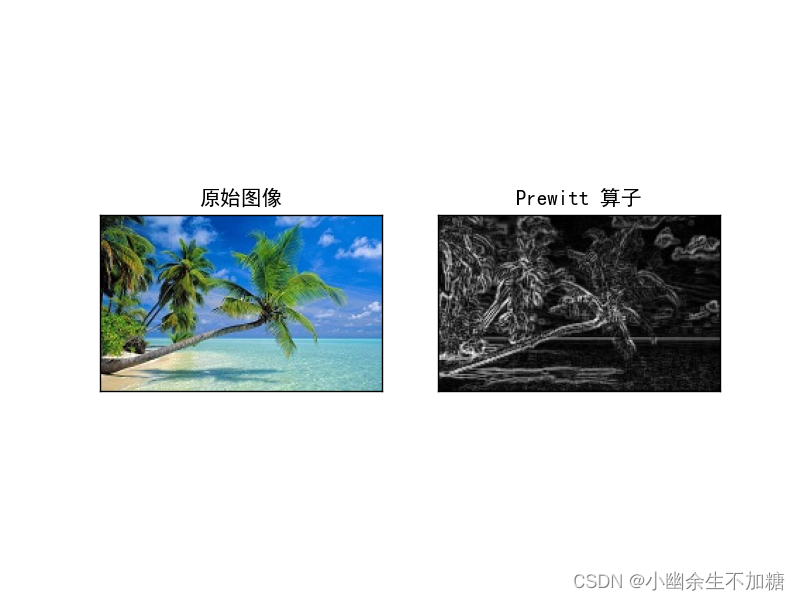
4. Prewitt operator edge detection

Prewitt edge operator is an edge template operator. The template operator is composed of an ideal edge operator image. The edge template is used to detect the image in turn. The template most similar to the detected area gives the maximum value. The Prewitt operator is similar to Sobel, using the grayscale of the upper and lower, left and right neighboring points of the pixel. The difference reaches the extreme value at the edge to detect the edge. It has a smoothing effect on noise and the positioning accuracy is not high enough.

The Prewitt_X operator actually performs non-normalized mean smoothing on the image in the vertical direction first, and then performs the difference in the horizontal direction; however, the Prewitt_Y operator actually performs non-normalized mean smoothing on the image in the horizontal direction first. Then perform vertical differentiation. This is why the Prewitt operator can suppress noise. In the same way, we can also get the Prewitt operator on the diagonal.

Code example:

import cv2 as cv
import numpy as np
import matplotlib.pyplot as plt

# 读取图像
img = cv.imread('test.jpg', cv.COLOR_BGR2GRAY)
rgb_img = cv.cvtColor(img, cv.COLOR_BGR2RGB)

# 灰度化处理图像
grayImage = cv.cvtColor(img, cv.COLOR_BGR2GRAY)

# Prewitt 算子
kernelx = np.array([[1,1,1],[0,0,0],[-1,-1,-1]],dtype=int)
kernely = np.array([[-1,0,1],[-1,0,1],[-1,0,1]],dtype=int)

x = cv.filter2D(grayImage, cv.CV_16S, kernelx)
y = cv.filter2D(grayImage, cv.CV_16S, kernely)

# 转 uint8 ,图像融合
absX = cv.convertScaleAbs(x)
absY = cv.convertScaleAbs(y)
Prewitt = cv.addWeighted(absX, 0.5, absY, 0.5, 0)

# 用来正常显示中文标签
plt.rcParams['font.sans-serif'] = ['SimHei']

# 显示图形
titles = ['原始图像', 'Prewitt 算子']
images = [rgb_img, Prewitt]

for i in range(2):
    plt.subplot(1, 2, i + 1), plt.imshow(images[i], 'gray')
    plt.title(titles[i])
    plt.xticks([]), plt.yticks([])
plt.show()

Output result:

5.LoG operator edge detection

The LoG edge detection operator was jointly proposed by David Courtnay Marr and Ellen Hildreth (1980). Therefore, it is also called edge detection algorithm or Marr & Hildreth operator. This algorithm first performs Gaussian filtering on the image, and then finds its Laplacian (Laplacian) second-order derivative, that is, the image and the Laplacian of the Gaussian function are filtered.

Finally, the edges of the image or object can be obtained by detecting zero crossings of the filtering results. Therefore, it is also referred to as the Laplacian-of-Gaussian (LoG) operator in the industry.

Code example:

import cv2 as cv
import matplotlib.pyplot as plt

# 读取图像
img = cv.imread("test.jpg")
rgb_img = cv.cvtColor(img, cv.COLOR_BGR2RGB)

gray_img = cv.cvtColor(img, cv.COLOR_BGR2GRAY)

# 先通过高斯滤波降噪
gaussian = cv.GaussianBlur(gray_img, (3, 3), 0)

# 再通过拉普拉斯算子做边缘检测
dst = cv.Laplacian(gaussian, cv.CV_16S, ksize=3)
LOG = cv.convertScaleAbs(dst)

# 用来正常显示中文标签
plt.rcParams['font.sans-serif'] = ['SimHei']

# 显示图形
titles = ['原始图像', 'LOG 算子']
images = [rgb_img, LOG]

for i in range(2):
    plt.subplot(1, 2, i + 1), plt.imshow(images[i], 'gray')
    plt.title(titles[i])
    plt.xticks([]), plt.yticks([])
plt.show()
 

This algorithm first performs Gaussian filtering on the image, then finds the second-order derivative of Laplacian, and detects the boundary of the image based on the zero-crossing point of the second-order derivative, that is, the image is obtained by detecting the zero crossings of the filtering result. or the edge of an object. The LoG operator actually combines Gauss filtering and Laplacian filtering. It first smoothes out noise and then performs edge detection.

Output result:

6. Canny operator edge detection

Canny edge detection is a method of detecting edges using a multi-level edge detection algorithm. In 1986, John F. Canny published the famous paper A Computational Approach to Edge Detection, which detailed how to perform edge detection. OpenCV provides the function cv2.Canny() to implement Canny edge detection.

step:

Use Gaussian filter to smooth the image and eliminate noise;
calculate the gradient intensity and direction of each pixel in the image;
use Non-Maximum Suppression to eliminate spurious responses caused by edge detection;
use dual threshold detection (Double Threshold) to determine real and potential edges;
edge detection is finally completed by suppressing isolated weak edges.

6.1 Apply Gaussian filter to remove image noise

Since image edges are very susceptible to noise interference, in order to avoid detecting erroneous edge information, the image usually needs to be filtered to remove noise. The purpose of filtering is to smooth some non-edge areas with weak texture in order to obtain more accurate edges. In actual processing, Gaussian filtering is usually used to remove noise in images.

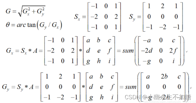
6.2 Calculate gradient

Here, we focus on the direction of the gradient, which is perpendicular to the direction of the edge. The edge detection operator returns Gx in the horizontal direction and Gy in the vertical direction. The magnitude G and direction Θ of the gradient (expressed as angle values) are:

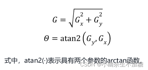
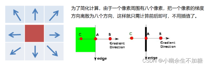
The direction of the gradient is always perpendicular to the edge, and the nearest values ​​are usually 8 different directions: horizontal (left, right), vertical (up, down), diagonal (upper right, upper left, lower left, lower right).

Therefore, when calculating the gradient, we will get two values ​​​​of the magnitude and angle of the gradient (representing the direction of the gradient).

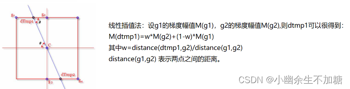
6.3 Non-maximum suppression

After obtaining the magnitude and direction of the gradient, traverse the pixels in the image and remove all non-edge points. In the specific implementation, the pixels are traversed one by one to determine whether the current pixel is the maximum value of the surrounding pixels with the same gradient direction, and whether to suppress the point is decided based on the judgment result. As can be seen from the above description, this step is an edge refinement process.

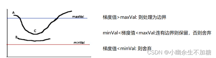
6.4 Applying dual thresholds to determine edges

After completing the above steps, the strong edges within the image are already within the currently acquired edge image. However, some virtual edges may also be within the edge image. These virtual edges may be generated by real images or due to noise. For the latter, it must be eliminated.

Set two thresholds, one of which is the high threshold maxVal and the other is the low threshold minVal. According to the relationship between the gradient value of the current edge pixel (referring to the gradient amplitude, the same below) and the two thresholds, the edge attributes are judged.

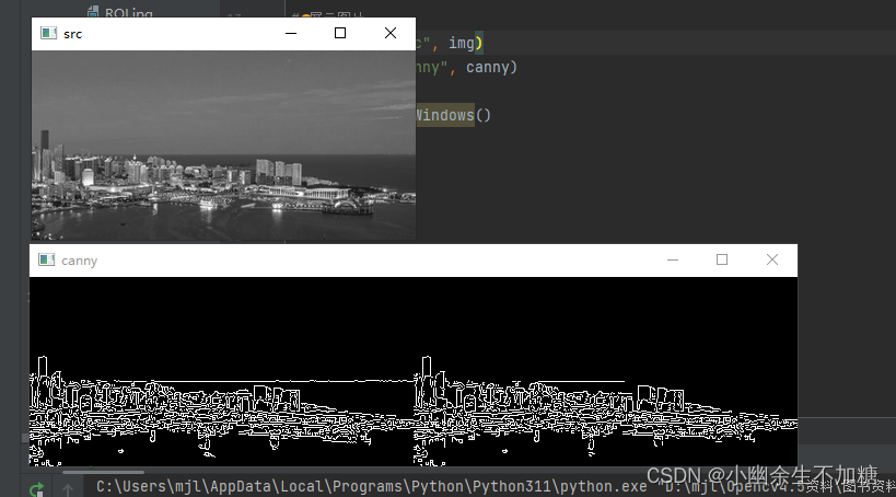
6.5 Code examples

import cv2
import numpy as np
# 读取图片, 并转换成灰度图
img = cv2.imread("test.jpg", cv2.IMREAD_GRAYSCALE)

# Canny边缘检测
out1 = cv2.Canny(img, 50, 150)
out2 = cv2.Canny(img, 100, 150)

# 合并
canny = np.hstack((out1, out2))

# 展示图片
cv2.imshow("src", img)
cv2.imshow("canny", canny)
cv2.waitKey(0)
cv2.destroyAllWindows()

Output result: