Using OT to solve crowd counting problems
Used OT+count loss + TV loss
to prove that the generalization error of OT is better than density map and Bayesian Loss
OT
Consider two distributions d\right\}_{i=1}^nX={
xi∣xi∈Rd}i=1n,Y = { yj ∣ yj ∈ R d } j = 1 n \mathcal{Y}=\left\{\mathbf{y}_j \mid \mathbf{y}_j \in \mathbb{R}^d\right \}_{j=1}^nY={
yj∣yj∈Rd}j=1n
Consider two measures μ , ν \boldsymbol{\mu},\boldsymbol{\nu}m ,ν ,1 n T μ = 1 n T ν = 1 \mathbf{1}_n^T \ball symbol{\mu}=\mathbf{1}_n^T \ball symbol{\nu}=11nTm=1nTn=1
任生成c : X × Y ↦ R + c: \mathcal{X} \times \mathcal{Y} \mapsto \mathbb{R}_{+}c:X×Y↦R+
Construct C ij = c ( xi , yj ) \mathbf{C}_{ij}=c\left(\mathbf{x}_i,\mathbf{y}_j\right)Cij=c(xi,yj)
Definition:Γ = { γ ∈ R + n × n : γ 1 = μ , γ T 1 = ν } \Gamma=\left\{\ball symbol{\gamma} \in \mathbb{R}_{+} ^{n \times n}: \ball symbol{\gamma} \mathbf{1}=\ball symbol{\mu},\ball symbol{\gamma}^T \mathbf{1}=\ball symbol{\nu}\right\ } }C={
c∈R+n×n:c 1=m ,cT 1=n }
OT:
W ( μ , ν ) = min γ ∈ Γ ⟨ C , γ ⟩ \mathcal{W}(\ballsymbol{\mu}, \ballsymbol{\nu})=\min _{\gamma \in \Gamma }\angle\mathbf{C}, \gamma\angleW ( μ ,n )=γ∈Γmin⟨C,c ⟩
W ( μ , ν ) = max α , β ∈ R n ⟨ α , μ ⟩ + ⟨ β , ν ⟩ s.t. α i + β j ≤ c ( x i , y j ) , ∀ i , j \begin{aligned} \mathcal{W}(\boldsymbol{\mu}, \boldsymbol{\nu}) & =\max _{\boldsymbol{\alpha}, \boldsymbol{\beta} \in \mathbb{R}^n}\langle\boldsymbol{\alpha}, \boldsymbol{\mu}\rangle+\langle\boldsymbol{\beta}, \boldsymbol{\nu}\rangle\\ &\quad \text { s.t. } \alpha_i+\beta_j \leq c\left(\mathbf{x}_i, \mathbf{y}_j\right), \forall i, j \end{aligned} W ( μ ,n )=α , β ∈ Rnmax⟨ a ,m ⟩+⟨ b ,n ⟩ st ai+bj≤c(xi,yj),∀i,j
DM-count
Let the predicted density map be z ^ ∈ R + n \hat{\mathbf{z}}\in\mathbb{R}_+^nz^∈R+n
gtThe density map of z ∈ R + n \mathbf{z}\in\mathbb{R}_+^nz∈R+n
count loss
The role of count loss here: because OT calculates the normalized density map, it has no quantity information.
ℓ C ( z , z ^ ) = ∣ ∥ z ∥ 1 − ∥ z ^ ∥ 1 ∣ \ell_C(\mathbf{z}, \hat{\mathbf{z}})=\left|\| \mathbf{z}\|_1-\| \hat{\mathbf{z}} \|_1 \right|ℓC(z,z^)=∣∥z∥1−∥z^∥1∣dimensional z , z ^ ≥ 0 , \mathbf{z},\hat{\mathbf{z}}\ge 0
,z,z^≥0 , _
_
_ {z}})=\left|\sum _{i=1}^n \mathbf{z}_i-\sum _{i=1}^{n}\hat{\mathbf{z}}_i\right|ℓC(z,z^)=∣∑i=1nzi−∑i=1nz^i∣
OT loss
ℓ O T ( z , z ^ ) = W ( z ∥ z ∥ 1 , z ^ ∥ z ^ ∥ 1 ) = ⟨ α ∗ , z ∥ z ∥ 1 ⟩ + ⟨ β ∗ , z ^ ∥ z ^ ∥ 1 ⟩ \ell_{O T}(\mathbf{z}, \hat{\mathbf{z}})=\mathcal{W}\left(\frac{\mathbf{z}}{\|\mathbf{z}\|_1}, \frac{\hat{\mathbf{z}}}{\|\hat{\mathbf{z}}\|_1}\right)=\left\langle\boldsymbol{\alpha}^*, \frac{\mathbf{z}}{\|\mathbf{z}\|_1}\right\rangle+\left\langle\boldsymbol{\beta}^*, \frac{\hat{\mathbf{z}}}{\|\hat{\mathbf{z}}\|_1}\right\rangle ℓOT(z,z^)=W(∥z∥1z,∥z^∥1z^)=⟨ a∗,∥z∥1z⟩+⟨ b∗,∥z^∥1z^ Where
α ∗ , β ∗ \boldsymbol{\alpha }^*,\boldsymbol{\beta}^*a∗,b∗ is the optimal solution to the dual problem of OT.
The cost matrix isc ( z ( i ) , z ^ ( j ) ) = ∥ z ( i ) − z ^ ( j ) ∥ 2 2 c(\mathbf{z} (i), \hat{\mathbf{z}}(j))=\|\mathbf{z}(i)-\hat{\mathbf{z}}(j)\|_2^2c(z(i),z^(j))=∥z(i)−z^(j)∥22
∂ ℓ O T ( z , z ^ ) ∂ z ^ = β ∗ ∥ z ^ ∥ 1 − ⟨ β ∗ , z ^ ⟩ ∥ z ^ ∥ 1 2 \frac{\partial \ell_{O T}(\mathbf{z}, \hat{\mathbf{z}})}{\partial \hat{\mathbf{z}}}=\frac{\boldsymbol{\beta}^*}{\|\hat{\mathbf{z}}\|_1}-\frac{\left\langle\boldsymbol{\beta}^*, \hat{\mathbf{z}}\right\rangle}{\|\hat{\mathbf{z}}\|_1^2} ∂z^∂ℓOT(z,z^)=∥z^∥1b∗−∥z^∥12⟨ b∗,z^⟩
One thing to note is that in the code, its OT loss is
ℓ O T ( z , z ^ ) = ⟨ ∂ ℓ O T ( z , z ^ ) ∂ z ^ , z ^ ⟩ \ell_{O T}(\mathbf{z}, \hat{\mathbf{z}})= \left\langle \frac{\partial \ell_{O T}(\mathbf{z}, \hat{\mathbf{z}})}{\partial \hat{\mathbf{z}}}, \hat{\mathbf{z}}\right\rangle ℓOT(z,z^)=⟨∂z^∂ℓOT(z,z^),z^⟩
https://github.com/cvlab-stonybrook/DM-Count/issues/29
To solve OT, use the most primitive sinkhorn (without log-domain
TV loss
This is mainly to stabilize the results
ℓ T V ( z , z ^ ) = ∥ z ∥ z ∥ 1 − z ^ ∥ z ^ ∥ 1 ∥ T V = 1 2 ∥ z ∥ z ∥ 1 − z ^ ∥ z ^ ∥ 1 ∥ 1 \ell_{T V}(\mathbf{z}, \hat{\mathbf{z}})=\left\|\frac{\mathbf{z}}{\|\mathbf{z}\|_1}-\frac{\hat{\mathbf{z}}}{\|\hat{\mathbf{z}}\|_1}\right\|_{T V}=\frac{1}{2}\left\|\frac{\mathbf{z}}{\|\mathbf{z}\|_1}-\frac{\hat{\mathbf{z}}}{\|\hat{\mathbf{z}}\|_1}\right\|_1 ℓTV(z,z^)= ∥z∥1z−∥z^∥1z^ TV=21 ∥z∥1z−∥z^∥1z^ 1
result
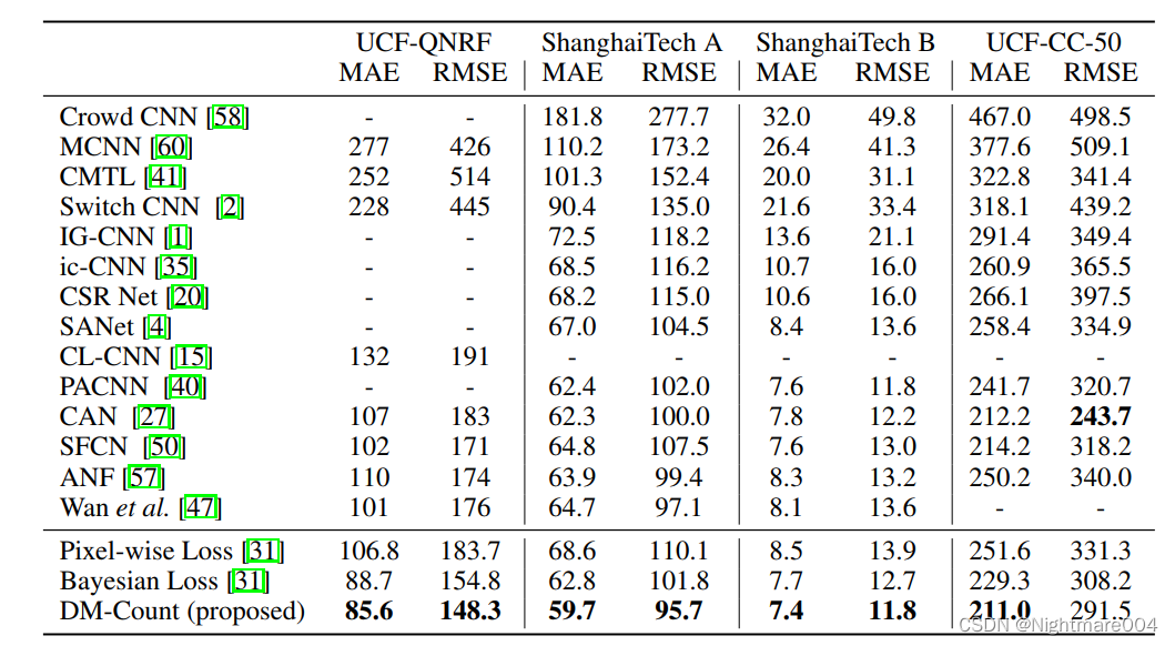
On UCF-QNRF
author model: mae 85.76006602669905, mse 150.3385868782564
I ran: best_model_7.pth: mae 89.24010239104311, mse 155.59441664755747