Disclaimer: Resale and reselling of the author's original code is prohibited, and violators will be prosecuted!
The idea for this issue's article comes from a three-high paper in the "Journal of Vibration Testing and Diagnosis" . Click the link to jump. "Three High" Paper Recommendations || Rolling bearing fault diagnosis method based on EEMD singular value entropy . Currently, this paper has been cited 58 times in CNKI statistics.

The abstract of the article is as follows:
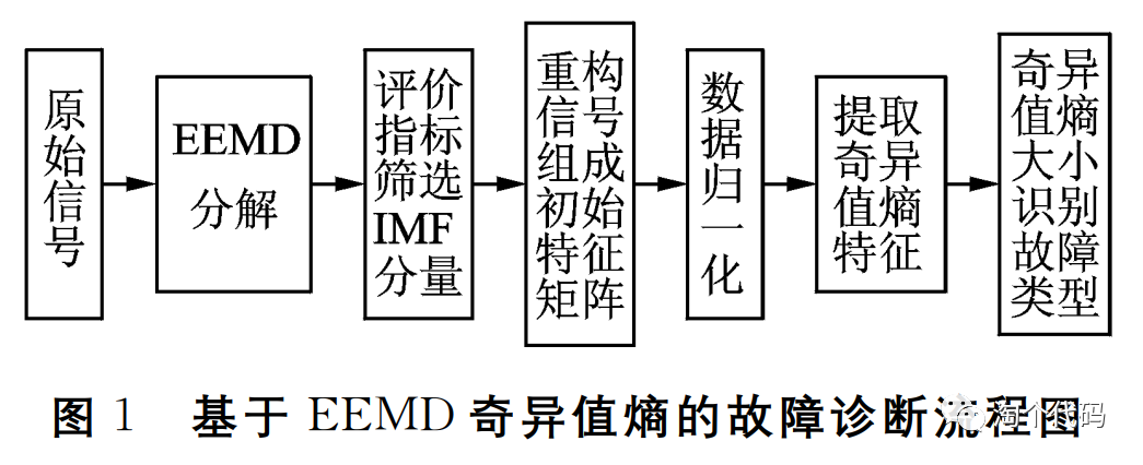
In order to make full use of vibration signals for fault identification, a rolling bearing fault diagnosis method based on ensemble empirical mode decomposition (EEMD) singular value entropy criterion is proposed. First, the vibration signal of the rolling bearing is decomposed by EEMD to obtain several intrinsic mode functions (IMF), and based on an evaluation index of the fault information content of the IMF component (i.e., kurtosis, mean square error and Euclidean distance ) to select the components that can represent the original signal state for signal reconstruction; secondly, use singular value decomposition technology to process the reconstructed signal, and combine the information entropy algorithm to obtain its singular value entropy; finally, use the magnitude of singular value entropy to determine the rolling bearing fault category. The results of verifying the method using vibration signals of rolling bearings from Western Reserve University in the United States show that compared with the traditional EMD singular value entropy fault diagnosis method, this method can clearly divide the category characteristic intervals of different working states of rolling bearings, and has higher performance. fault diagnosis accuracy.
The process is as follows:
This article will use MATLAB code to strictly restore all simulation results mentioned in the paper ! A perfect reproduction of the main methods of this paper ! First look at the code directory: all codes are .m files, not encrypted .p files!

Next, each step will be explained based on the screenshot above:
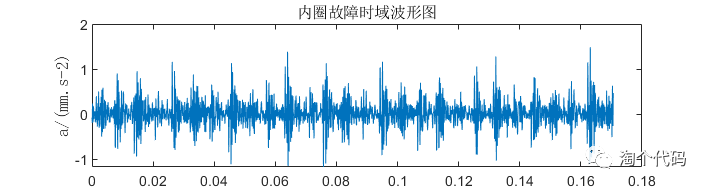
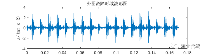
Step 1: Draw the time domain waveform diagram - corresponding to Figure 2 of the paper
The data selected in the paper are four state data at 1797 rotational speed in the bearing failure data set of Western Reserve University, which are normal, inner ring failure, rolling element failure, and outer ring failure. Corresponding to 97, 105, 118 and 130.mat respectively.
First draw the time domain waveform of each state, and run the plotfigure.m file in the first step to get the following picture:


Step 2: EEMD decomposition + drawing of 3 indicators - corresponding to Figures 3 and 4 of the paper
This article takes the rolling element failure 118.mat as an example to explain. EEMD decomposition diagram:
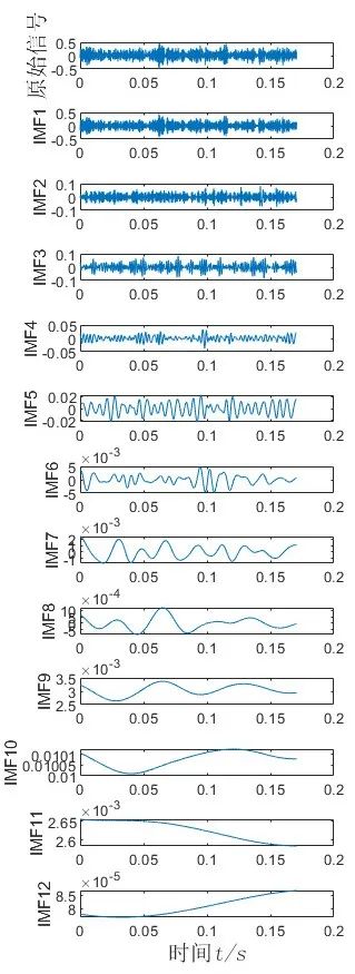
In order to select the real IMF components that can reflect fault information and extract effective fault features, this paper proposes an evaluation method for true and false IMF components based on kurtosis, mean square error and Euclidean distance.
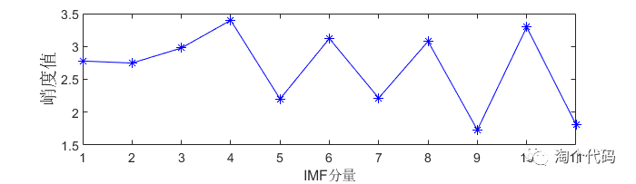
The kurtosis plot of the IMF component:
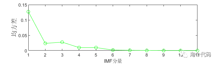
IMF component mean square error plot:
IMF component Euclidean distance diagram:
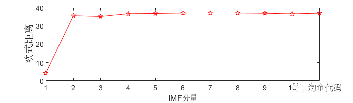
The three evaluation indicators of each IMF component decomposed by the rolling element fault signal EEMD are shown in the above three figures. It can be found from the figure that the kurtosis and mean square error of the first three components among the 12 IMF components are larger than those of other components; in the Euclidean distance between each IMF component and the original signal, starting from the third IMF component, it tends to level. It can be seen from the properties of the three evaluation methods that the first three IMF components in the figure contain rich fault information and can characterize the working condition of the rolling bearing, which provides guarantee for the reliability of extracting the singular value entropy of the initial feature matrix in the next step. Therefore, the first three IMF components are selected for signal reconstruction and subsequent singular value entropy calculation.
Step 3: Data processing + signal reconstruction
The second step has shown that the first three IMF components can be used to characterize the bearing state. The paper selects 20 sets of data for each state, but the paper does not say how many sample points are used for each set of data.
Here, Xiaotao still follows previous articles and selected 2048 sampling points for each state.
There are 4 states in total, each state has 20 sets of samples, and the data size of each sample is: 1×2048. Then perform EEMD decomposition on the 20*4*2048 data group by group.
Because the article will be compared with EMD decomposition later in the article, EMD decomposition is also performed here in the third step.
Run the shujuchuli_1797.m file to get two files, cg.mat and emd_cg.mat, where cg.mat is the data obtained by EEMD decomposition, and emd_cg.mat is the data obtained by EMD decomposition.
Step 4: Singular value entropy diagnosis - corresponding to Figure 5 of the paper
Copy the two data cg.mat and emd_cg.mat obtained in the third step to the fourth step, and run SVDMAIN.m to directly perform singular value decomposition on all state samples of the two data, and obtain the singular value entropy and plot . The result is as follows:


It can be seen from the figure that due to the shortcomings of EMD decomposition itself, the difference in singular value entropy containing fault information obtained after different signal decomposition is small, making the singular value entropy intervals of the four states of the rolling bearing fuzzy, making it difficult to distinguish fault categories; In the EEMD decomposition, it can be seen that there are significant differences in singular value entropy between different fault categories of rolling bearings. Compared with the traditional EMD singular value entropy method, the EEMD singular value method can distinguish fault categories more clearly.
Each of the four states of rolling bearings belongs to an interval range, and the category intervals have no intersection, as shown in Table 1. This result shows that the criterion of EEMD singular value entropy can accurately distinguish the fault categories of rolling bearings.
Notice! Students who can see this seriously may wish to replace the EEMD method in this article with other data decomposition methods to try, or replace the singular value entropy in this article with the entropy of other decomposition methods. Maybe this is also a good paper. What a way!
Partial code sharing
clc
clear
close all
fs=12000;%采样频率
Ts=1/fs;%采样周期
L=2048;%采样点数
t=(0:L-1)*Ts;%时间序列
STA=1; %采样起始位置


load 97.mat
X = X097_DE_time(1:L)'; %这里可以选取DE(驱动端加速度)、FE(风扇端加速度)、BA(基座加速度),直接更改变量名,挑选一种即可。
figure
plot(t,X); %故障信号
ylabel('a/(mm.s-2)','fontsize',10,'fontname','宋体');
title('正常时域波形图')
set(gcf,'unit','centimeters','position',[10 2 15 4])


load 105.mat
X = X105_DE_time(1:L)'; %这里可以选取DE(驱动端加速度)、FE(风扇端加速度)、BA(基座加速度),直接更改变量名,挑选一种即可。
figure
plot(t,X); %故障信号
ylabel('a/(mm.s-2)','fontsize',10,'fontname','宋体');
title('内圈故障时域波形图')
set(gcf,'unit','centimeters','position',[10 4 15 4])


load 118.mat
X = X118_DE_time(1:L)'; %这里可以选取DE(驱动端加速度)、FE(风扇端加速度)、BA(基座加速度),直接更改变量名,挑选一种即可。
figure
plot(t,X); %故障信号
ylabel('a/(mm.s-2)','fontsize',10,'fontname','宋体');
title('滚动体故障时域波形图')
set(gcf,'unit','centimeters','position',[10 6 15 4])


load 130.mat
X = X130_DE_time(1:L)'; %这里可以选取DE(驱动端加速度)、FE(风扇端加速度)、BA(基座加速度),直接更改变量名,挑选一种即可。
figure
plot(t,X); %故障信号
ylabel('a/(mm.s-2)','fontsize',10,'fontname','宋体');
title('外圈故障时域波形图')
set(gcf,'unit','centimeters','position',[10 8 15 4])
Each code has detailed comments, and all pictures mentioned in the article can be run! Just follow the steps in the article and run them one by one.
05 code acquisition
How to obtain the complete code: Click below to read the original text, or reply with keywords in the background, case-insensitive:
tgdm830