1. Introduction to 4D-Label technology
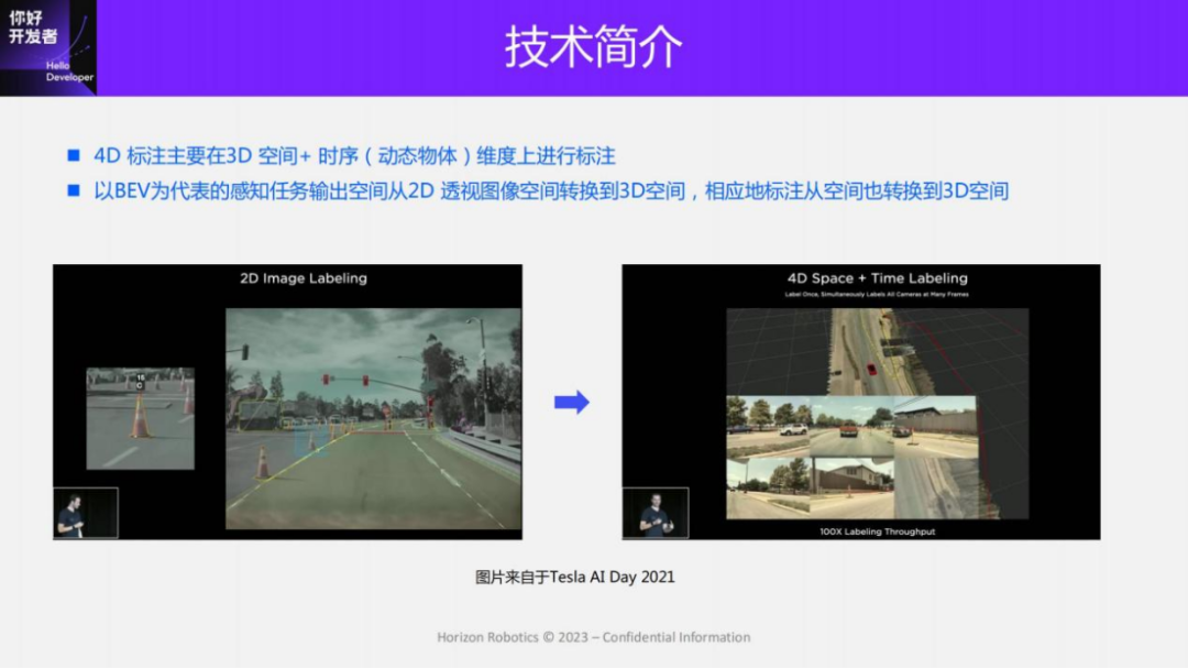
First, let’s introduce 4D-Label technology. 4D is mainly about 3D space and timing. A typical feature of perception technology represented by BEV is that the output space is converted from a 2D perspective image to a 3D space. Originally it was all in the image space, the input was the image, and the output was also the information in the 2D image pixel space, that is, what you see is what you get. However, the input of BEV perception technology is 2D images or 2D videos, and the output is the perception results of 3D space, usually some 3D static or dynamic results under the vehicle body coordinate system. For BEV perception, the generation of true value data is a very critical link, because the annotated space needs to be converted from 2D perspective image space to 3D space. Among them, considering the time-series dynamic objects, a very important technology that needs to be used is 4D reconstruction technology.
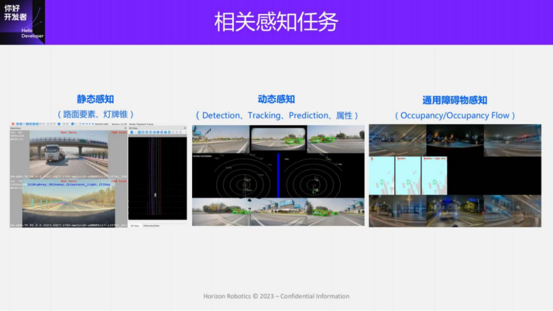
Some of the perception tasks involved in this technology sharing can be roughly divided into three categories: The first category is static perception. The output form of static perception is actually more and more like a local high-precision map, including physical layer, logical layer and semi-dynamic layer. Among them, the physical layer mainly includes continuous elements of the road surface such as lane lines, discrete elements of the road surface such as road identifiers, and static elements in the air such as light signs. The semi-dynamic layer mainly includes objects that are easily moved, such as cones and barrels. The logical relationships are mainly lane link relationships, as well as the relationship between road elements and traffic lights. Dynamic perception is mainly about moving vehicles and pedestrians, including detection, tracking, and prediction, as well as some attributes of speed and acceleration. Some existing end-to-end perception frameworks can directly complete all the above perception outputs in the same network. Another type of task is general obstacle perception, which is mainly aimed at non-whitelisted objects in the scene. The current mainstream perception tasks in the industry are Occupancy and Ocupancy Flow. The basic principle of this type of task is to divide the space into regular voxels. Predicting the occupation of each voxel and the speed of each voxel is essentially a geometric method rather than a semantic method to achieve the recognition of universal objects. Today we will mainly introduce some labeling solutions for these three types of tasks.
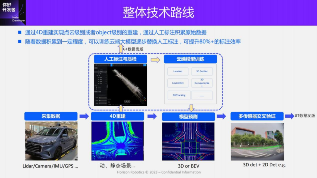
The overall technical route of 4D-Label is consistent whether it is a multi-mode solution for collection scenes or a pure visual solution for mass production data. The overall idea is: first collect data, and then perform point cloud or Object-level 4D reconstruction. On the basis of obtaining the 4D reconstruction space, manual annotation and quality inspection are carried out through 3D annotation tools, and then the release of the true value data is completed. With more and more manually labeled data, some large models can be trained in the cloud to assist in labeling, improve labeling efficiency, and reduce labeling costs. When the data scale on the cloud accumulates to a certain level, the performance of the cloud model will be greatly improved. At this point, most annotation tasks can be automated.
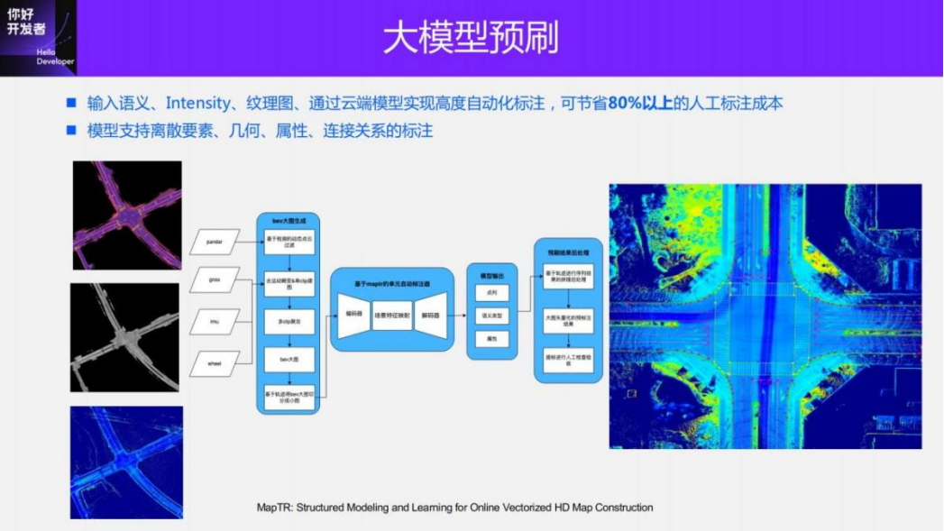
In addition, in order to further improve the quality and automation of annotation, we will design some automatic quality inspection strategies. For example, multi-sensor cross-validation is used to pre-brush large models on 2D images to obtain some annotation results. At the same time, the annotation results are compared with the annotation results in 3D space to remove data with large differences and only retain annotations with good consistency. data as true values, thereby ensuring the quality of true value data. By pre-brushing large models, we can currently save more than 80% of the annotation manpower through this strategy, and even some annotations like dynamic objects can be fully automated.
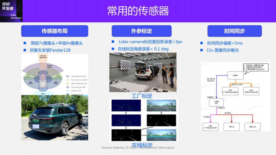
The hardware foundation involved in 4D annotation is, first of all, the layout of the sensor. In autonomous driving solutions above L2++, a peripheral view + surround view layout is usually adopted, forming a two-layer 360-degree imaging range. If it is a collection vehicle oriented to collection scenes, Pandar128 Lidar will generally be installed on the roof for labeling.
After obtaining the modified vehicle, external parameter calibration and time synchronization between sensors must be performed to achieve spatio-temporal consistency of data between different sensors. The external parameter calibration involved mainly includes the calibration between Lidar and camera, as well as the calibration between GPS, IMU and Vcs coordinate system. Calibration methods can be divided into two types, one is factory calibration and the other is online calibration. Factory calibration is a relatively comprehensive and systematic calibration performed at the factory. High-precision calibration results are obtained through specific labeling tools, but calibration cannot be performed frequently. Online calibration is to use the sensing results of some terminals to perform external parameter calibration. Online calibration can be performed at high frequency and can effectively ensure the lower limit of sensor accuracy. For example, when the sensor position changes due to jitter, online calibration can obtain Latest calibration results. In the actual process, we will use both methods. After the external parameters of the sensor are obtained through factory calibration, real-time or scheduled updates are performed through online calibration.
After obtaining the external parameter calibration, time synchronization between multiple sensors is also required to ensure accurate data correlation between different sensors. In our solution, 11V image synchronization exposure is used, and the time deviation is less than 5ms.
In addition, let’s introduce the definition of some data formats involved in our solution. Two basic data concepts are involved here.
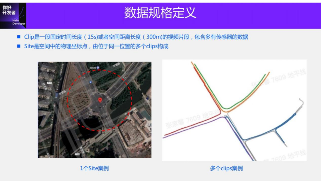
The first data concept is Clip. Clip is a piece of data video, which can be a fixed length or a fixed spatial distance. For example, during mass production, the length of the Clip can be set to 15s. In acquisition mode, spatial distance can be used, limiting it to local segments of 300m. Each clip contains data from multiple sensors. For example, in acquisition mode, clip contains Lidar point cloud data, 11V image data, and data from all sensors such as GPS, IMU, and wheel speedometer.
The second data concept is Site. Site is a physical coordinate point in space, which can be understood as a GPS point in space. This spatial location has a unique characteristic. A Site can contain multiple Clips passing through it. As a simple example, if you define the center point of an intersection as a Site, you can filter out all Clip data passing through the intersection through the GPS range.
2. Multi-modal annotation scheme for collection scenarios
The above is a brief technical introduction to some 4D-Label. Next, I will introduce two solutions: one is a multi-mode annotation solution for collection scenes, and the other is a pure visual solution for mass production. The multi-mode labeling solution adds Pandar128 radar to the mass-produced perception sensor. Annotation solutions for mass production mainly use data collected by mass-produced sensors for annotation. Our solution is purely visual perception, so only image information (combined with inertial navigation, wheel speedometer, etc.) is used for annotation. For some mass production solutions with Lidar, Lidar can be used to reduce the difficulty of dynamic labeling.
The first is the multi-mode solution. We will introduce the labeling process according to these tasks:
We introduce the multi-modal labeling scheme according to the three tasks of static, dynamic and general obstacles.
The first is the annotation of static pavement elements. The annotation of static pavement elements is essentially modeling of the pavement, that is, local mapping. In our solution, single-pass reconstruction and multi-pass aggregation are used. This method can, on the one hand, improve the efficiency of mapping and share the cost of labeling; on the other hand, it can also ensure the integrity of mapping and improve recall and long-distance true values.
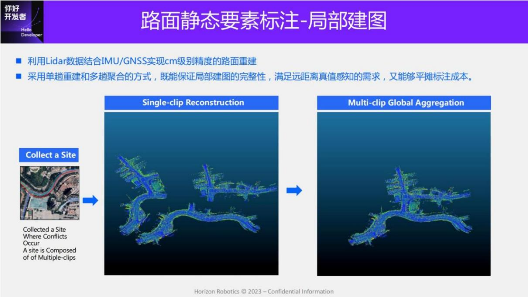
Let me introduce the specific plan: First, use the data collected by Pandar128, combined with IMU and GNSS data, to perform a single-trip reconstruction to obtain a single-trip point cloud map; each clip corresponds to a point cloud map, and then all clips located at the same site are reconstructed. Collect the point cloud maps, establish the correlation between clips, determine the joint optimization paradigm, and aggregate the point cloud maps of multiple clips to obtain a complete local map.
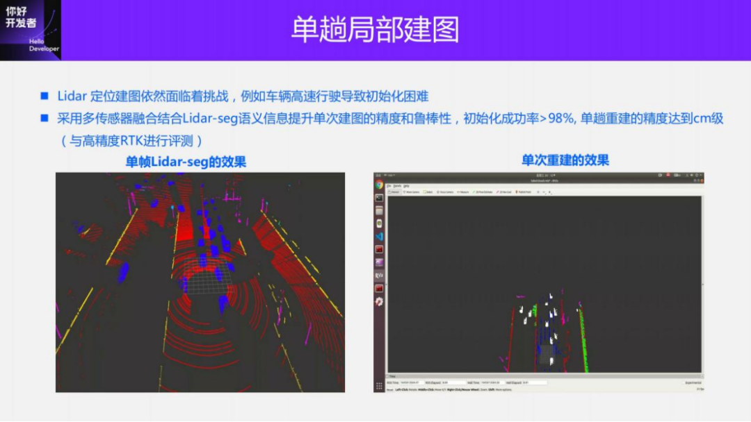
In our plan, we need to meet the needs of mapping in three scenarios: urban areas, highways, and parking. These environments present very big challenges. We have made some optimizations for single-pass local mapping. For example, the initialization of high-speed scenes can easily fail due to too fast speed, single environment, and insufficient feature constraints. Our solution introduces semantic information to provide more accurate correspondence between Lidar key points and also uses data from multi-sensors such as wheel speedometers and GNSS to assist initialization. After these optimizations, the success rate of initialization can be increased to more than 98%, and the reconstruction accuracy of a single pass can reach centimeter level (evaluated with the high-precision Novatel).
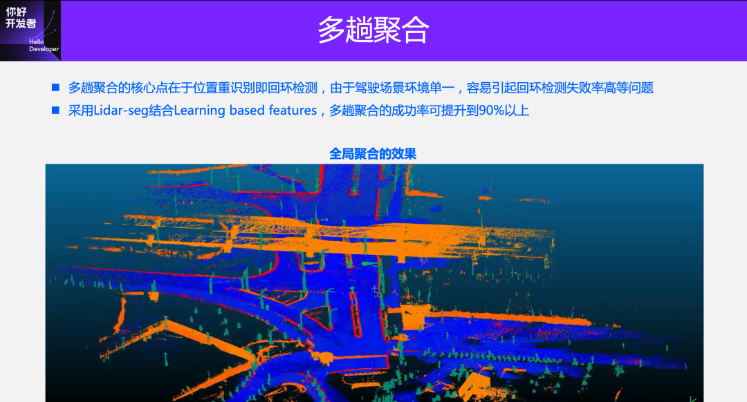
After obtaining a single trip reconstruction, in order to improve the integrity of the local map and improve the recall of road surface elements, the results of multiple clip reconstructions need to be aggregated. The core point of multi-pass aggregation is location re-identification, which is loopback detection in SLAM. The key to loopback detection is to provide feature-level correspondence. However, because this scene is relatively simple, such as a high-speed scene or an intersection scene, there are not many features that can be effectively identified, which can easily lead to loopback detection failure or relatively large deviations.
In response to these problems, we have made some optimizations to aggregation: first, like single-trip reconstruction, some semantic information is introduced, which can obtain some significant features of road surfaces and signboards, and use semantic information to guide matching; in addition, we also use Some learning methods and some key points obtained can provide more robust matching results in some extreme environments. Through these two strategies, the success rate of multi-pass reconstruction can reach more than 90%. The demo below is the effect of a local map after global aggregation. It can be seen that because the accuracy of mapping is high enough, the element structure of the road surface on the lidar intensity map is particularly clear.
The reflectivity of Lidar is sensitive to materials. When encountering special materials, worn-out roads, or water accumulation, the road elements on the intensity map will be unclear and difficult to identify. On the other hand, the intensity of Pandar128 itself needs to be calibrated. The same unit Lidar sensors may experience instability in intensity when traveling across the sky or across locations. In order to improve the recall of annotations, our solution introduces semantic maps and texture maps to provide more information (see the figure above).
Texture images mainly achieve Pixel-level fusion through external parameter calibration of Lidar and vision, and finally obtain the reconstruction results of road texture. Texture images can provide very rich information. In theory, as long as the data in the scene with driving conditions are met , texture images can be annotated. Like the texture map, the semantic map is obtained by using the perception results of 2D images through the fusion of Lidar-camera. The introduction of the perception results can handle some weak texture situations.
When annotating, we project the data of three different modalities onto a plane to obtain a large picture of the BEV space, and obtain the true value data through manual annotation. Since the projection process retains height information, the annotation results can use this height information to obtain 3D space data.
After accumulating a certain amount of data, we use the data to train a large cloud model for auxiliary annotation. The model adopts our own work MapTR. The input is the information of large images in three modalities, and the output is directly instance-level data. Each lane line will be represented as an ordered sequence of points, which saves a lot of post-processing. These annotated results can be used to obtain training samples through simple processing. In the future, we will also try to use MapTR to directly mark the logical layer.
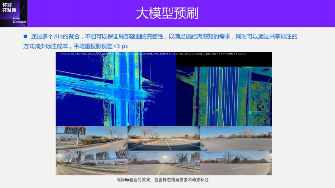
This is a labeling case we made through a multi-mode solution. There are three clips in this case, and the different colored tracks in the upper left corner represent different clips. Through the aggregation of three clips, the integrity of the intersection is ensured. Because in some cases where intersections are relatively large, single-trip collection and reconstruction cannot guarantee that the intersection can be completely reconstructed. Through the aggregation of multiple Clips, the integrity of the intersection can be ensured, while also meeting the true value requirements for long-distance sensing.
In addition, through aggregation, the cost of clip annotation can also be shared equally. Because after aggregation, a large BEV picture only needs to be annotated once to generate the true values of all clips. We evaluate the multi-mode ground truth by projecting the annotated ground truth into the image space and calculating the reprojection error. Our solution can achieve a reprojection error of less than 3 pixels.
Our solution has advantages in many aspects compared with HDmap positioning to generate ground truth. The first is strong scalability. High-precision maps produced by map dealers use expensive sensors when constructing maps. The cost is very high and the scalability is relatively poor. This is reflected in the fact that the coverage rate of high-energy maps is not very high, especially in urban areas. Although our solution is based on collection vehicles, we also need to consider the scalability of the collection fleet, so we use sensors with general accuracy. In addition, the main purpose of the maps created by map dealers is for positioning and navigation, so complete mapping is required. The primary purpose of 4D-Label is for labeling. The first thing to consider for sensory data is quality, quantity and Diversity, so there is no need to do complete map reconstruction or even map maintenance. It only needs to do sampling reconstruction in some areas to meet the demand for true value diversity.
This is the first difference. The second difference is that the map of the map dealer is updated slowly due to the freshness. This will lead to the need to invest a lot of human resources to identify inconsistencies between the map and the actual scene when generating true values. In most cases, 4D-Label can be built and used immediately, and there is no need to consider the issue of freshness.
In addition, there will be differences in positioning accuracy. The current high-precision map positioning method based on visual perception has a lateral error of about 10-20cm and a longitudinal error of more than 30-40cm. With such accuracy, the deviation is already larger than one lane line, and there is no way to meet the demand for true value accuracy. The 4D-Label method does not need to consider the global positioning accuracy, but only needs to ensure the local odometry accuracy, so its accuracy will be relatively high. The horizontal and vertical errors can be less than 10cm. This is some comparison between map providers HD Map and 4D-Label. All in all, the primary goal of 4D annotation is to meet the perceived truth-value requirements, and all solution designs should be centered around meeting the quantity, quality, and diversity of truth-value data.
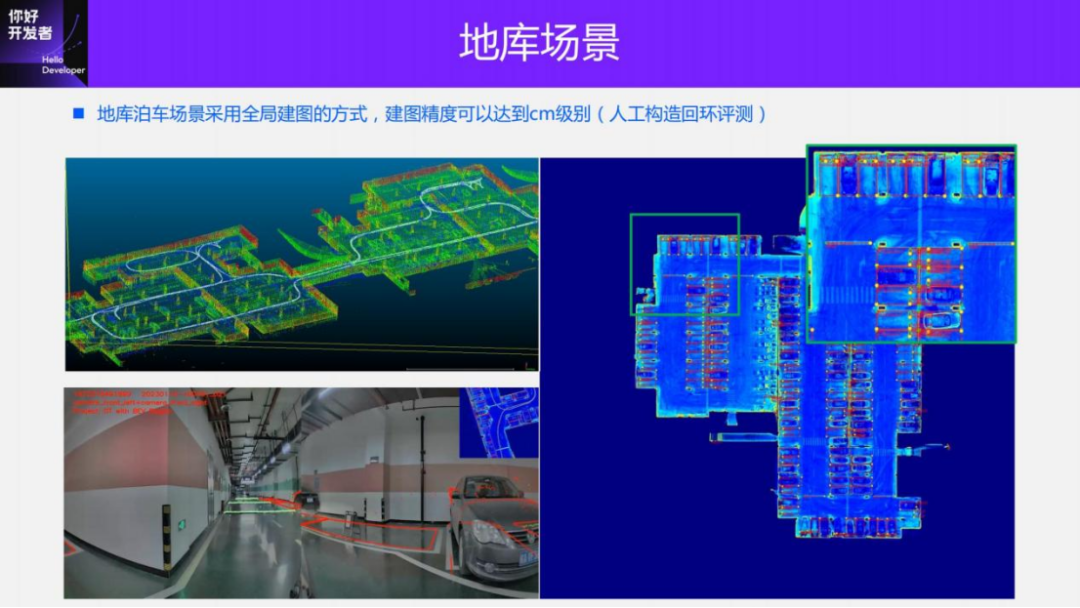
What I just talked about was driving. For labeling in the parking scene, the underlying mapping scheme is basically the same. The only difference is that in the basement parking scenario, there is no GNSS information, and the method of multi-pass reconstruction + global aggregation cannot be used. Therefore, in the parking scene, we use the full scene mapping method to completely reconstruct the map from the collected data. The optimization strategy for improving mapping accuracy is basically the same as that for driving. It mainly uses Lidar-seg semantic information to impose some constraints. The accuracy of parking scene reconstruction can reach 4-5cm. We mainly conduct evaluation by artificially constructing loopbacks. When labeling, we also developed corresponding pre-brushed large models. The detection of basement points, limiters, warehouse corners and walls are now all carried out through pre-brushing of large models.
The above introduction is the annotation of static elements of the road surface, and then the annotation of dynamic objects will be introduced. The annotation of dynamic objects adopts the Lidar+vision post-fusion solution. The main process is that first there is a large model for Lidar detection, which senses the input Pandar128 point cloud data and obtains the detection frame of the 3D object on the point cloud of each frame. Then the traditional Kalman filtering method is used to track the perception results between different frames to obtain the tracking results of each object, so that a complete trajectory of each object in time series can be obtained.
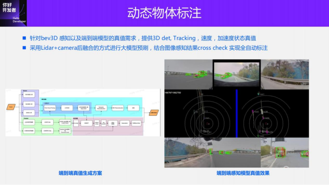
By using the self-vehicle trajectory obtained by Lidar SLAM, each moving object can be projected into the global coordinate system to obtain the global trajectory. Afterwards, further optimization of the trajectories of these moving objects, such as the smoothness of the trajectories and dynamic constraints, can lead to smoother and more accurate trajectories. After getting the trajectory of the moving object, you can get all its information, including track ID, predicted information, speed and acceleration and other attributes. After obtaining this information, we can generate true values for dynamic perception tasks, such as detection, prediction, and end-to-end direct estimation of speed and acceleration attributes.
The biggest advantage of the 4D annotation process on the cloud is that future information can be used for annotation. In other words, a moving object can use its future information to assist the current labeling, and therefore can obtain a relatively high precision or recall. As we mentioned earlier, there will be time synchronization between vision and Lidar, and the vision 11V image is exposed at the same time, and there will be a time deviation in the scanning between it and Lidar. Using time synchronization information and trajectory information, the motion information of the object can be interpolated to any moment, thereby obtaining the true value of each moment. For example, when there is a missed detection on some Lidar frames, the results on that frame can be supplemented by the time series trace difference.
In order to further improve the quality of true values, we use 2D pre-brushing of large models and compare them with 3D interpolation results to achieve automatic quality inspection. Only the 3D projection results that have a relatively high overlap with 2D will be retained as high-quality true values, otherwise they will be discarded. Doing so will not affect the effect of the true value, because each training sample in the detection task is an object, not an image. Therefore, even if some objects in the same sample, image or frame are not completely accurately labeled, it will not affect the final training task. If we can ensure that 60% -70% of the true values in an image at a moment are accurately annotated, it can meet the needs of model training. Another use of this projection method is to assign 2D perceptual attributes to the 3D annotation results, such as the door opening and closing of the vehicle, the color of the lights, etc. Information that is difficult to identify through Lidar can be obtained through 2D images.
Next, we will introduce the annotation of other static elements, such as traffic lights, traffic signs and cones in driving scenes. The labeling scheme of these objects is basically the same as that of dynamic objects. The main difference lies in two points: the acquisition method of the 3D space bounding box and the tracking method. Here we take the cone barrel scheme as an example to introduce.
Our main route: First, we have a large model of Lidar segmentation, using the semantic information of Lidar to extract the potential 3D proposal of the cone bucket, but there may be a lot of noise; then we use the time series information to detect the 2D cone bucket. The results are tracked and correlated; finally, the 2D cone barrel is used to correlate with the 3D-proposal to remove some noise. It can be seen that the final labeling scheme actually relies more on the 2D cone-barrel detection model, and its accuracy also depends on the 2D cone-barrel large model. Finally, through 2D and 3D cross-validation, the labeling results of the cone barrel are obtained. Our solution can achieve a cone-barrel labeling accuracy rate higher than 95%, and a ranging error of less than 5% within a 50m range.
This demo shows some ground-truth annotation effects in two scenarios, one is a parking scene and the other is a driving scene. For some cases where 2D detection is detected but 3D is missing, the flag can be marked as ignore and will not participate in the training.

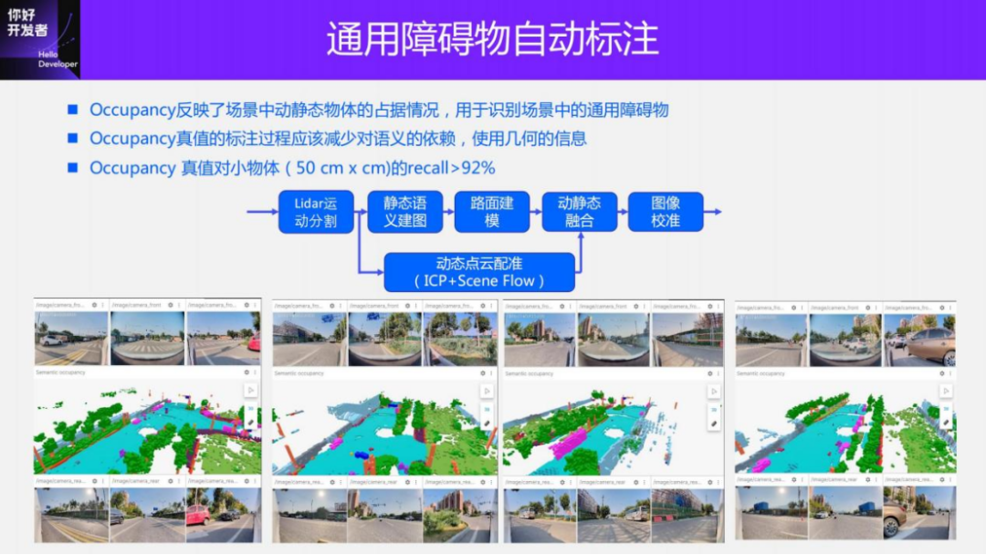
Finally, let’s introduce the automatic labeling of general obstacles, which is actually the perception task of Occupancy and Occupancy flow in driving. Occupancy reflects the occupation of dynamic and static objects in the scene. It divides the space into uniform voxels. Places occupied by objects are marked as 1, and places occupied by no objects are marked as 0. In addition, each voxel also has a velocity vector information, which represents the movement of the voxel, that is, Occupancy flows. Occupancy and Occupancy flow actually perform 4D reconstruction of the scene. Its main advantage is that it can identify some common, non-whitelisted obstacles in the scene, such as some scattered stones, scattered irregular objects, and other obstacles such as Pets, cars on the wrong side of the road, etc.
The existing Occupancy also has some true value generation solutions, as well as some public data sets. This year, CVPR held an Occupancy competition and also released a data set. However, the main problem with these existing solutions is that they rely too much on semantic information. For example, when dividing the scene into dynamic and static, it will be done through 3D detection, which introduces strong semantic information. In fact, in the process of true value generation, relying too much on whitelist objects will lead to the actual generated true value, which cannot truly fulfill the original purpose of universal object detection.
In response to this situation, we have made some improvements to Occupancy's solution. The main idea is to minimize reliance on semantics throughout the process. When separating static and dynamic motion, we do not rely on whitelist information, but use geometric information for motion segmentation. After segmentation, the static scene and the dynamic scene are divided and conquered. For the static scene, the static semantic mapping method introduced earlier is used to obtain the static point cloud; for the dynamic scene, the Scene Flow or ICP method is mainly used to register the dynamic point cloud. , and finally obtain a 4D point cloud of the entire scene. At the same time, when generating each frame of image, we will also do a cross check between the image and the 3D result, and finally generate the true value.
Below are some cases. There are many obstacles in this scene, such as irregularly placed and temporary traffic lights. There are also pet dogs and strollers pushed by pedestrians. Pet dogs like this one can be identified better. There are also some irregularities, such as temporary traffic lights placed at intersections, which can also be easily identified. We made some quantitative evaluations on the performance of Occupancy ground truth. For small objects such as 50cm×50cm, the accuracy rate is higher than 92%.
3. Pure visual annotation solution for mass production scenarios
Next, I will introduce a purely visual annotation solution for mass production scenarios.
A purely visual annotation solution mainly uses vision plus some data from GPS, IMU and wheel speedometer sensors for dynamic and static annotation. Of course, for mass production scenarios, it doesn’t have to be pure vision. Some mass-produced vehicles will have sensors like solid-state radar (AT128). If we create a data closed loop from the perspective of mass production and use all these sensors, we can effectively solve the problem of labeling dynamic objects. But there is no solid-state radar in our plan. Therefore, we will introduce this most common mass production labeling solution.
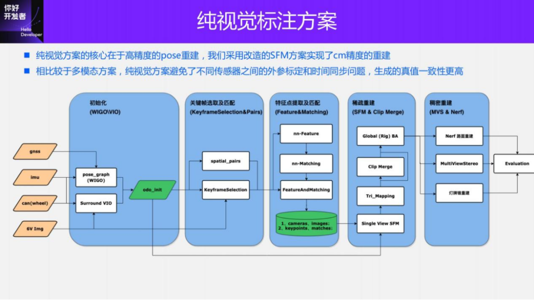
The core of a purely visual annotation solution lies in high-precision pose reconstruction. We use the Structure from motion (SFM) pose reconstruction scheme to ensure reconstruction accuracy. However, traditional SFM, especially incremental SFM, is very slow, and the computational complexity is O(n^4), where n is the number of images. This kind of reconstruction efficiency is unacceptable for large-scale data annotation. We have made some improvements to the SFM solution.
The improved clip reconstruction is mainly divided into three modules: 1) Using multi-sensor data, GNSS, IMU and wheel speedometer, construct pose_graph optimization to obtain the initial pose. This algorithm is called Wheel-Imu-GNSS-Odometry ( WIGO); 2) Feature extraction and matching of the image, and triangulation directly using the initialized pose to obtain the initial 3D points; 3) Finally, a global BA (Bundle Adjustment) is performed. On the one hand, our solution avoids incremental SFM, and on the other hand, parallel operations can be implemented between different clips, thus greatly improving the efficiency of pose reconstruction. Compared with the existing incremental reconstruction, it can achieve 10 to 20 times efficiency improvement.
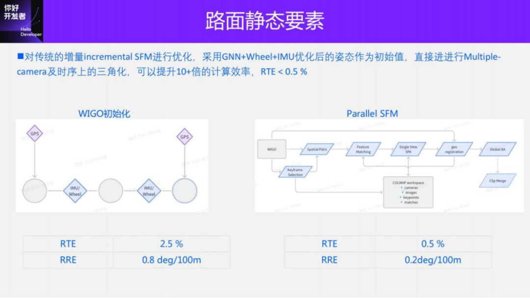
The picture above shows that these are the two important modules WIGO and Parallel SFM just introduced. The first is a multi-sensor fusion algorithm that provides an initialization pose, and the second is a parallel SFM reconstruction algorithm. WIGO's Relative Translation Error (RTE) indicator can reach 2.5%, and Relative Rotation Error (RRE) can reach 0.8deg/100m. After introducing visual observation, the RTE index of Parallel SFM can be reduced to 0.5%, and the RRE index can be reduced to 0.2deg/100m. (All indicators are compared with the results of Lidar Odometry).
During the single reconstruction process, our solution also made some optimizations. For example, we use Learning based features (Superpoint and Superglue), one is feature points and the other is matching method, to replace the traditional SIFT key points. The advantage of learning NN-Features is that on the one hand, rules can be designed in a data-driven manner to meet some customized needs and improve the robustness in some weak textures and dark lighting conditions; on the other hand, it can improve Efficiency of keypoint detection and matching. We have done some comparative experiments and found that the success rate of NN-features in night scenes will be approximately 4 times higher than that of SFIT, from 20% to 80%.
After obtaining the reconstruction result of a single Clip, we will aggregate multiple clips. Different from the existing HDmap mapping scheme that uses vector structure matching, in order to ensure the accuracy of aggregation, we use feature point level aggregation, that is, the aggregation constraints between clips are implemented through feature point matching. This operation is similar to loop closure detection in SLAM. First, GPS is used to determine some candidate matching frames; then, feature points and descriptions are used to match images; finally, these loop closure constraints are combined to construct a global BA (Bundle Adjustment) and optimize. At present, the accuracy and RTE index of our solution far exceed some of the current visual SLAM or mapping solutions.
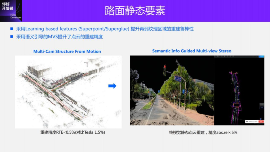
This slide shows a site reconstruction case. The left image is the reconstruction result of Paralle SFM, and the right image is the reconstruction result of dense point cloud. The reconstruction of dense point cloud uses the traditional MVS solution, but combines semantic information. As can be seen from the reconstruction results on the right, the reconstructed semantic point cloud will be very accurate because there is no problem of time synchronization between Lidar and camera across sensors and sensor jitter. It can even be directly annotated on the point cloud. Lane segmentation.
It should be noted that our main purpose of reconstructing dense point clouds is to verify the accuracy of SFM reconstruction. In the actual annotation process, dense point cloud reconstruction of the entire scene will not be performed. MVS reconstructs pixel-by-pixel, which is very resource-intensive and very costly. However, most of the reconstructed point clouds are non-interest areas. In order to save costs and improve labeling efficiency, we will design different labeling solutions for different perception tasks.

First, let’s introduce the ground-truth annotation scheme for perception schemes such as lane lines, curbs, and pavement markings for pavement elements. The core of pavement static element annotation lies in the reconstruction of 3D pavement. Our reconstruction plan is mainly based on SFM and using Nerf for road reconstruction. We use Nerf to express the road surface. When performing Nerf query, input the coordinate point of the BEV space, enter it into the corresponding MLP after encoding, and finally output the height, RGB and semantic results of the point. During the Nerf initialization process, we use Parallel SFM reconstruction to provide two types of information: one is the pose information of the camera corresponding to each image, and the other is some reconstructed sparse 3D points. By extrapolating the camera's pose point, the initial 3D shape of the road surface can be obtained, which is used as the initialization of the road surface height.
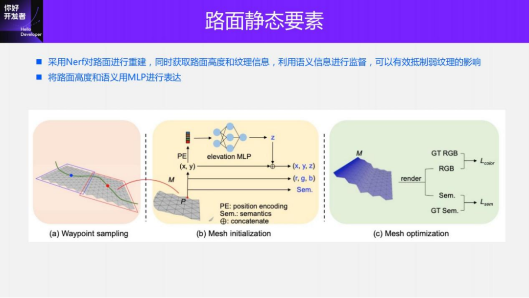
There are two main types of supervision information for Nerf training, one is RGB and the other is 2D semantic map. Among them, semantic information can reduce the influence of weak texture. The training process is also a query process. For each point in the space, send it to Nerf and you will get some returned height values, returned RGB values and semantic values. After obtaining this information, it can be projected into different 2D perspective images and semantic image spaces according to the pose provided by SFM to form a supervised loss and optimize Nerf. After Nerf converges, the same query process is performed to obtain the reconstructed 3D road surface results.

This is the effect of reconstructing a partial site. The picture on the left is composed of multiple clips, and each track line of a different color corresponds to a clip. By aggregating multiple clips, a complete reconstruction of the intersection can be obtained. In order to verify the accuracy of reconstruction, we project the reconstruction results onto the original image. It can be seen that the consistency of the projection is very high. The results obtained from the visual reconstruction are not affected by jitter between heterogeneous sensors, and the semantic segmentation results projected onto the original image and 2D are basically aligned. We made some simple evaluations on the results of road surface reconstruction and calculated the reprojection error of lane lines. The accuracy can reach an error of less than 3 pixels.
The picture on the right is a partial enlargement, showing some reconstruction details. From the picture, you can see that the fonts on the road reconstructed by Nerf are clearly visible. The reconstruction details are already very exquisite. If annotation is done on it, the efficiency of annotation will be greatly improved.
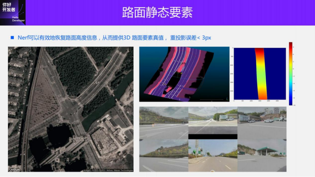
Another example shown is the reconstruction of a sloped road surface. This slope is data from Chongqing. This slope is about 10 meters. Through the Nerf reconstruction solution, the real road geometry can also be restored relatively well. On the right is a reconstructed elevation map, from blue to red, indicating increasing height. It can be seen that the entire slope is relatively short in the middle and relatively high on both sides, which also reflects the rationality of the reconstruction results. With the height information, the lane lines marked on the road slope can be perfectly aligned with the lane lines on the image. The reprojection result on the lower right side confirms this result.
The picture on the left shows the comparison between Nerf reconstruction results and satellite images. It can be seen that the overall spatial position and shape are also very consistent. In the initial stage of annotation, we import the road reconstruction results into the annotation tool for annotation. After accumulating a certain amount of data, we can train a large cloud model for auxiliary annotation to improve annotation efficiency.
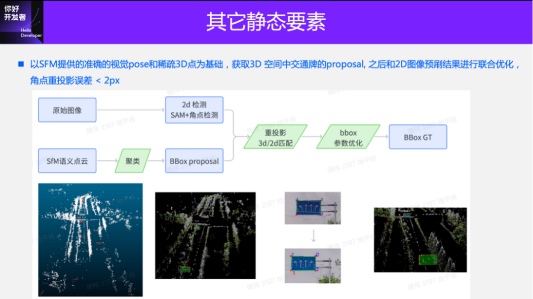
Next, we will introduce the annotation of other static elements, such as the annotation of traffic signs, traffic lights and cones. The labeling schemes for these three types of objects are basically the same. Here we take traffic signs as an example to introduce the labeling schemes for these static elements.
The true value generation of signboards, like the road surface, also relies on the initial pose of the camera and the initial 3D points provided by Parallel SFM. At the same time, we use 2D detection or Segment Anything Model (SAM) to process the 2D image to obtain the corner points of the traffic sign. It should be noted that the method of obtaining corner points will be more suitable for traffic signs than the detection results. For a simple example, a rectangular sign, projected onto the image, will be a polygon. The traditional 2D detection method, Failure to fit perfectly, or resulting in deviations in reconstruction.
Using the camera pose and 3D sparse points provided by Parallel SFM, we can easily determine the 3D-2D correspondence and the tracking relationship in 2D time series. Then we can construct a triangulation optimization paradigm and adjust the corner points of the traffic signs in the 3D space. The position and orientation of the traffic sign usually need to be ensured by the rectangular constraints to minimize the reprojection error of the corner points in the 2D image space.

This is the reconstruction of a sign projected onto the original image. It can be seen that when projected, it is basically completely self-consistent with the motion of the vehicle. There will be no major deviation due to vehicle jitter. The multi-mode solution will have very obvious jitter. This also shows that the 3D reconstruction results of traffic signs and the recovery of camera poses are very accurate.
The picture on the right is a visualization of the reconstruction result of the sign in 3D space. Putting the 3D signboard and the 3D sparse dots together, you can see that the fit is very good.
For pure visual reconstruction solutions, we mainly evaluate them in two ways: one is to evaluate pose indicators, such as using Lidar odometry as the true value to evaluate the RRE and RTE indicators; the other is to evaluate by calculating the reprojection error. The former can evaluate the accuracy of reconstructed pose accuracy and scale, and the latter can evaluate the accuracy of pose accuracy and 3D reconstruction results. Using these two evaluation methods, the performance of the pure visual reconstruction scheme can be evaluated reasonably. Our cloud-based pure visual reconstruction solution has higher reconstruction accuracy than the current mainstream visual crowdsourcing mapping solution in the industry. Compared with multi-mode solutions, the precision level of multi-mode can be achieved in terms of accuracy.
Pure visual dynamic annotation solutions are very challenging, especially single-view pure visual solutions. The biggest challenge lies in the reconstruction of dynamic objects. Because moving objects do not comply with the traditional 3D multi-view geometric assumptions, it is difficult to pass traditional method for reconstruction. Some monocular (small overlap between peripheral viewing angles) ranging algorithms in the industry mainly use triangular ranging, which requires strong road geometry assumptions, real object size and accurate camera pose. These assumptions, which are difficult to satisfy in real scenarios, result in limited ranging accuracy and limited scenarios that can be satisfied, making them unable to be used to generate true values.
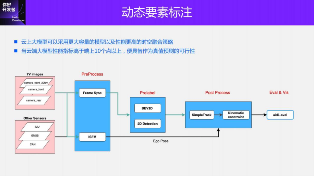
We use a large model + trajectory optimization method to label purely visual dynamic objects. First, we will train a BEV 3D detection model with larger capacity and higher performance on the cloud. The input of this model is an 11V image, and the output is the 3D BBox detection result of dynamic objects. Using this detection result combined with the pose information provided by the vehicle, you can use the multi-modal annotation scheme introduced earlier to project the dynamic objects into a unified global coordinate system, perform timing tracking and trajectory optimization, and finally generate detection, tracking, Predictions and true values of various attributes.
The same as the multi-mode solution, the optimized 3D inspection results will be projected onto the corresponding image, and cross-compared with the effect of the 2D inspection large model to achieve automatic quality inspection, and at the same time, more attributes can be obtained.
We explain the rationality of this solution from several aspects: 1) Although the ranging accuracy of the large visual model is difficult to achieve the effect of Pandar128 Lidar detection, the true values of these two models (the true values generated by pure visual dynamic annotation We call it the pseudo-true value) is close to the improvement performance of the on-device model, which we have verified in practice; 2) The cloud model has better cross-vehicle generalization, which means that it can be used with a small amount of The collection car maintains this large model to meet the pseudo-realistic needs of all production cars.
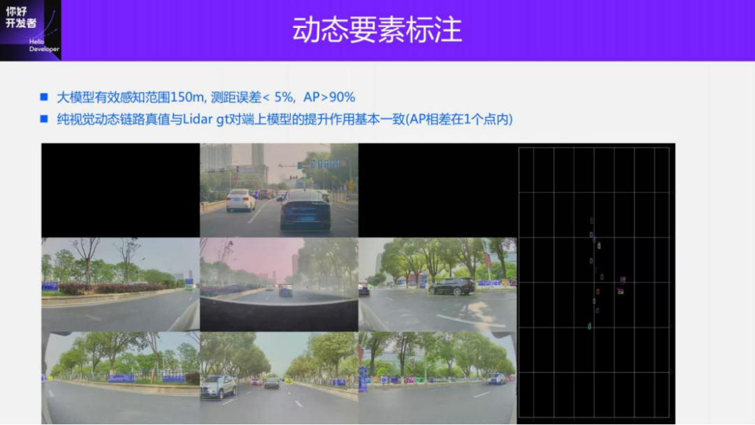
This is the effect of ground truth generated by our purely visual dynamic annotation scheme. As can be seen from the demo, the generated trajectory is very stable, the effective sensing range of the true value is 150m, the ranging error is less than 5%, and the AP is greater than 90%. At the same time, our solution supports different viewing angles (5v/6v/ 7v/11v) free switching. Our solution is currently being used in mass production.
We have also done some exploration into pure visual universal obstacle detection, that is, Occupancy perception. We now mainly use the Vidar solution for annotation. First, we obtain the depth map of each viewing angle through the monocular depth estimation solution, and then use the depth to convert it into a point cloud in the 3D space. After generation, the point cloud is voxelized to generate Occupancy. true value.
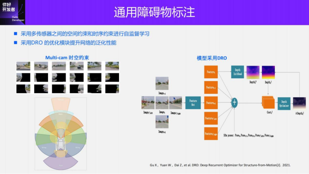
For monocular depth estimation, we use the DRO solution, but make some improvements based on the characteristics of our sensor layout. First, our scheme is self-supervised, and we adopt spatial constraints and timing constraints between multiple views for self-supervision. In terms of spatial constraints, there is actually some overlap between different cameras. Although it is relatively small, it can also constrain the training of this model and provide some scale information. For timing constraints, because of the SFM foundation, a more accurate camera pose can be obtained. Using this pose combined with the depth value can achieve self-supervision constraints on timing. It should be noted that spatial constraints can constrain dynamic objects, but timing constraints can only constrain static scenes.
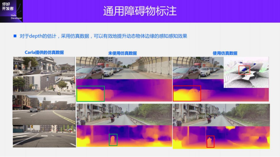
In addition, sharing a training trick and adding simulation data during the depth training process can improve the depth performance in discontinuous areas at the edge of the object. We added simulation data generated by the Carla simulator to the real training set. Although the visual difference between Carla's data and real data is quite far, during the experiment we found that using simulation data can effectively improve the perception of object edges. This is the result of an experiment we did. When simulation data is not used, you can see that the edges of the object are relatively blurry and even somewhat incomplete. But after using simulation data, the edges of these objects will become clearer, such as the edges of this cyclist. When the depth map is projected into the 3D space, it can be seen that the point cloud effect of the simulation data is not added, and the edges are over-smoothed, resulting in smearing. The depth of the edge of a real object is not continuous, so it is normal that it should have a very sharp effect. We found that after using simulation data, the edges can become clearer and more layered without smearing.
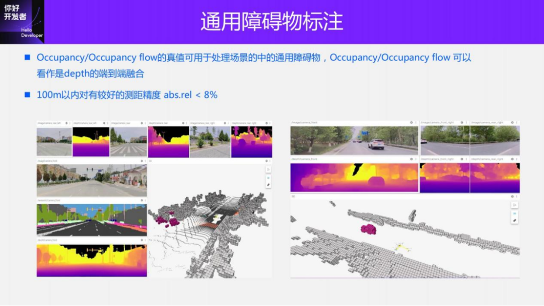
This is the ground-truth value of Occupancy generated by our visual scheme. Here we show two scenes, one is a rural road scene and the other is a traffic jam scene. It can be seen from the demo effect that the occupied situation reflected by the generated Occupancy true value is completely consistent with the real situation. It can be seen that the vehicles inside can still be identified relatively clearly. The relative relationships between congested vehicles, your vehicle's position, and congested obstacles are also correct. Our solution can achieve a range measurement error of less than 8% within 100m.
4. 4D-Label labeling operation platform
After introducing the purely visual annotation solution, we introduce Horizon’s 4D annotation cloud operation platform.
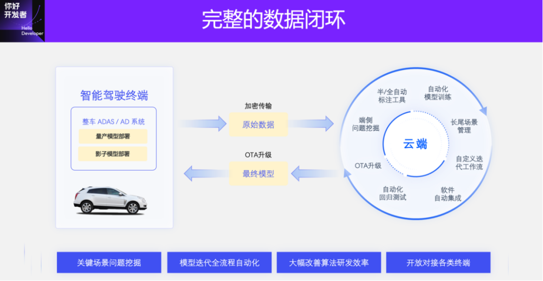
4D annotation is a very important module in the data closed loop. Data production and annotation are run on the cloud, and other modules together form a complete and efficient data closed loop system. After the data is returned and uploaded from the terminal to the cloud, similar data will be mined, a data set will be constructed, and then 4D annotation will begin. After obtaining the results of these annotations, the model will be automatically trained and updated.
Here I will mainly introduce the annotation tools, data mining methods and data links in the cloud.
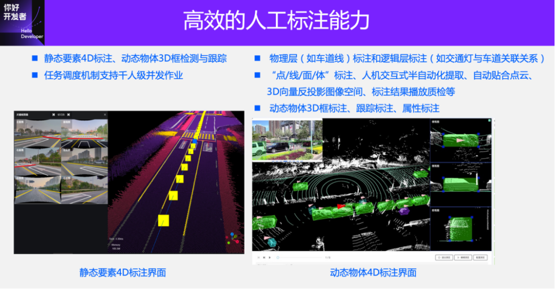
These are some static and dynamic annotation tools in 4D annotation. Although many of our solutions can be automated, visualization and annotation tools are still needed for data quality inspection and editing. Static annotation mainly refers to elements such as curbs, lane lines, road discrete elements and light sign cones; dynamic annotation mainly refers to the detection and tracking of dynamic objects. Static annotation tools have basic functions such as 3D visualization, perspective conversion, and real-time projection of 2D images of 3D annotation results to ensure the efficiency and accuracy of annotation.
In addition, we also improved the annotation efficiency of the tool by introducing some algorithms. For example, static annotation, because the bottom layer is a reconstructed camera pose, can produce a correlation between time and space. When annotating a 3D space, you can see its alignment with the image in 2D in real time. At the same time, you can also edit on the image to adjust the results in 3D space. In the dynamic annotation process, because there are sequential tracking results, only a small amount of manual participation is needed to generate the entire trajectory of the object in sequence. If there is a deviation in this trajectory, some adjustments can be made manually. After the adjustment, the entire system will automatically update all trajectories, which is very efficient. In addition, the annotation tool is developed based on the web, can support concurrent operations of thousands of people, and can meet the needs of large-scale data annotation.
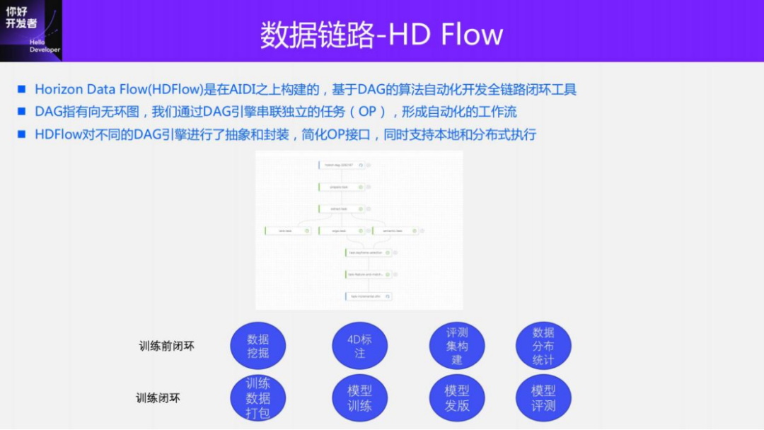
In order to automate the entire process, we also have a complete set of data link tools. The tool we are using internally now is called Horizon Data Flow (HDFlow). It mainly connects various tasks in series by constructing a directed acyclic graph, and each processed task is a node. For example, for 4D annotation tasks, data preprocessing, data pre-brushing, 4D reconstruction, large model pre-brushing and true value quality inspection, model release, manual annotation, and manual quality inspection are all task nodes. HDFlow can be connected in series to form a complete data link, and these nodes can run automatically. In this case, the efficiency of the entire process can be greatly improved.
Currently, the entire HD Flow supports some nodes, in addition to those mentioned last time, there are also pre-training links such as data mining, 4D annotation, construction of evaluation sets, statistics of data distribution, and some closed loops during the training process such as training data. Packaging, model training, model release and model evaluation.
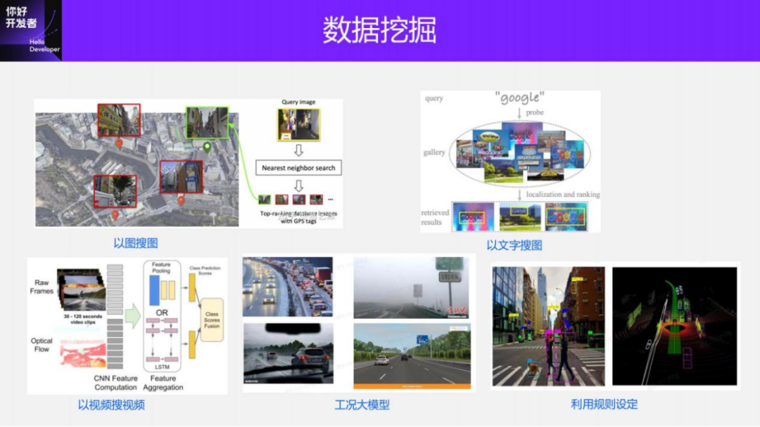
For a certain bad case, in order to quickly collect training data, we have developed a variety of data mining tools in the cloud. For example, if you search for images using images, you can use models to extract image features for certain specific cases and search historical data to obtain similar training data; you can search for images with text and search for videos with videos. Among them, the difference between searching for videos through videos and searching for pictures through pictures is that some timing clues can be added for data collection in some timing perception tasks. In addition, there are some large models of working conditions, which can be used for tagging or pre-brushing. Our solution can set some rules to mine data based on the pre-brush results. For example, after obtaining the pedestrian detection and tracking results, the pedestrian trajectory can be used to determine whether the pedestrian is at an intersection or on a straight road, and whether he is going straight or turning. Through these data mining solutions in the cloud, we can also obtain a large amount of needed data.
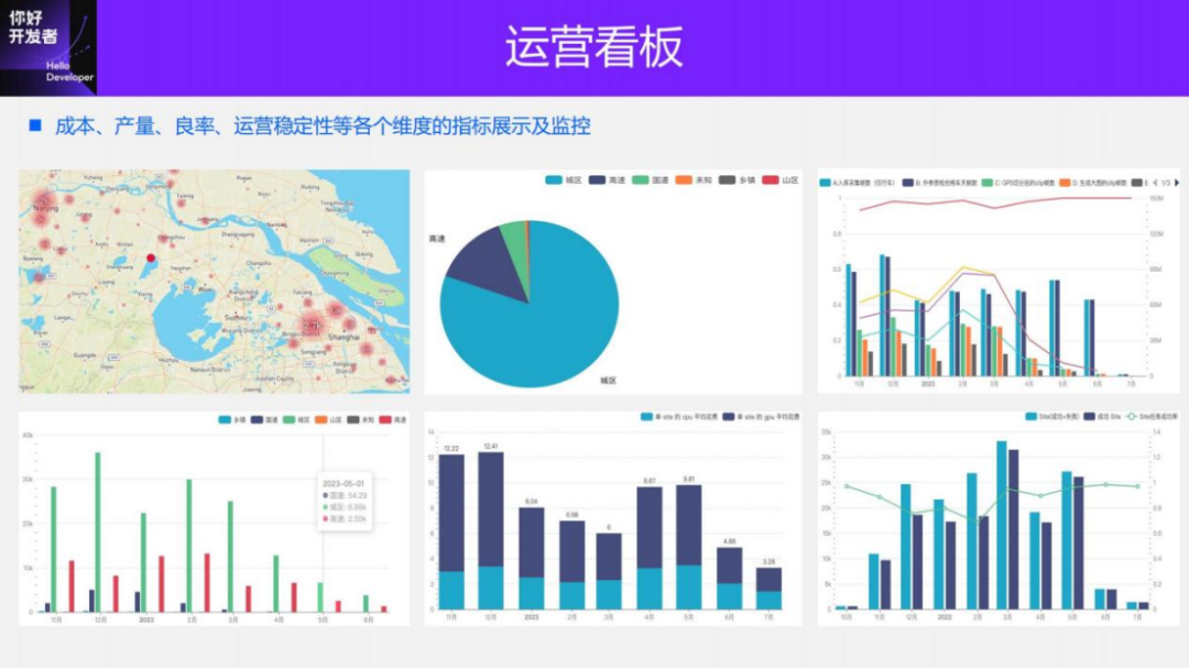
In order to better detect the efficiency and cost of 4D-Label annotation, we developed a complete set of dashboards to observe from various dimensions such as cost, output, yield, operating efficiency, and data validity. Through the dashboard, we can also see the location distribution, scene distribution and time distribution of true value generation. These distributions are very valuable for true values, especially static true values.
At the same time, we have also built a complete data lineage. From data return to annotation to model update, we can accurately track the data usage and processing status of each batch of data in each link in the middle, and digitally analyze the entire data. Operational costs are more precisely controlled and optimized.
5. 4D-Label development trends

Next, let me introduce the subsequent development trends of 4D-Label technology.
First, let’s introduce the relationship between 4D-Label and digital twins or data simulation. An important module of 4D-Label is to reconstruct the scene in 4D and obtain structured information (i.e., the labeled dynamic and static true values). The core module of data simulation lies in the construction of scene library. After obtaining a large number of scene libraries, synthesize new scenes according to certain rules. For example, after obtaining a certain scene, erase, add, and edit the vehicles and moving objects in the scene to obtain a new scene. The rendering of the scene obtains training samples, and structured data can also be obtained at the same time for various simulations, including control simulation, perception simulation, etc. Therefore, 4D-Label is equivalent to an important material library for data simulation.
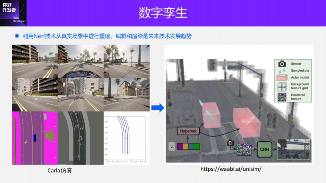
Through data simulation, we can solve many problems. And compared with traditional game engine simulation, it has more advantages in realism. What is shown on the left side of this picture is a simulation of a traditional game scene. Its scene is constructed directly through graphics, and its authenticity is very different from the real scene. The latest Unisim (CVPR2023) solution shown on the right is a better way to go through the process of scene reconstruction, synthesis and rendering. In other words, all its materials are reconstructed from real scenes and rendered through neural networks, so its visualization is more realistic than traditional emulators.
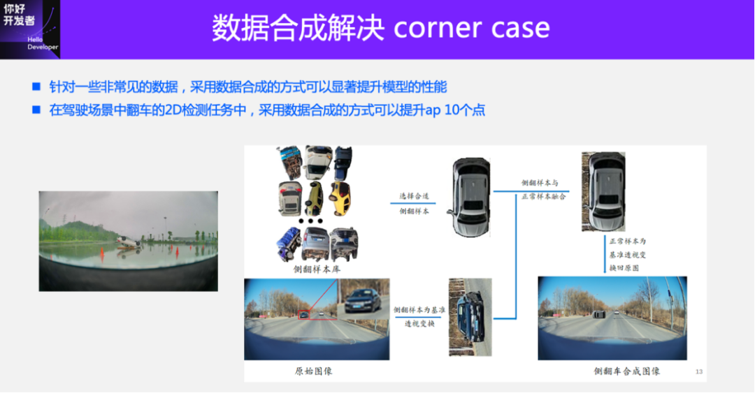
Simulation data can help us solve many practical problems in mass production. To give two examples, one is a pain point problem in intelligent driving scenarios—the corner case collection problem. In real scenes, such as rollovers in driving scenes, pets or pedestrians appearing on the highway, the data of these scenes is very difficult to collect and the cost is very high. Generating such training samples on a large scale through data synthesis is a very effective solution. Here I will give a 2D case to detect vehicles involved in accidents on the road, which is difficult to collect in practice. But once you have these foreground (rollover) materials, you can get the true value through simple image editing techniques. In the actual verification process, this method can also very effectively improve the performance of the task. This is a 2D task, what about 3D tasks? For example, to generate true values for some cones or barrels, or to create true values for sliding or rolling vehicles, we need to use 3D reconstruction technology to restore its underlying 3D geometry, including static scenes and dynamic vehicles. , and then merge these scenes together through data synthesis and rendering technology. Compared with full-scenario simulation, this solution is easier to implement and the effect is more obvious.
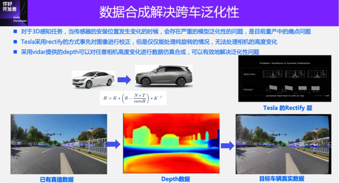
Another example to give is the generalization problem of straddling cars. In 3D perception tasks, changes in the size of the vehicle will cause changes in the installation position of the camera, which will seriously affect the performance of the 3D perception task. This will result in the data of many vehicles not being reusable and research and development costs remaining high. Using data simulation to solve the problem of cross-vehicle generalization, the main idea is to first reconstruct the 4D scene, including static reconstruction and dynamic reconstruction, and then simulate the sensors at different installation positions to generate true values. In this case, only a small number of collection vehicles are needed to collect data, and the true values of different sensor layouts can be automatically generated to achieve data reuse for different vehicles, thereby reducing research and development costs.
Here, we take another simple case, using Vidar to synthesize the true values of car models with different installation positions. How to reuse existing data when the shape of the vehicle changes. For example, because Tesla has a single model, it uses geometric correction (Homography transformation) to normalize the camera to the same plane. However, it has great limitations, that is, it can only solve the case where the camera is purely rotated, and when the camera has a height change, this correction method cannot meet the needs.
If the camera has height changes, it is necessary to obtain accurate depth information of the scene. Using the Vidar solution provided earlier, the true value of each pixel can be obtained. Although the depth value of the pixel is not very accurate, it is sufficient for changing the perspective and synthesizing a new perspective. In this way, it can be used to simulate generating new true values when the sensor changes. The method using Vidar is essentially a way to explicitly reconstruct the scene. Another solution is to use Nerf for reconstruction, which is an implicit reconstruction method that expresses the scene into MLP for reconstruction, editing and rendering. Compared with explicit reconstruction, which is more effective, the unisim solution introduced above falls into this category.
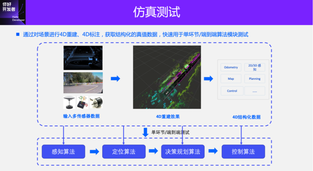
In addition, the true values generated by 4D-Label can be used for simulation tests in different aspects. After 4D Label reconstruction obtains the dynamic and static structured information in the scene, it can be input into the autonomous driving system to complete the simulation of each module, such as control simulation, positioning simulation, and perception simulation. The most difficult of these is perceptual simulation, which requires a high degree of realism in the input data.
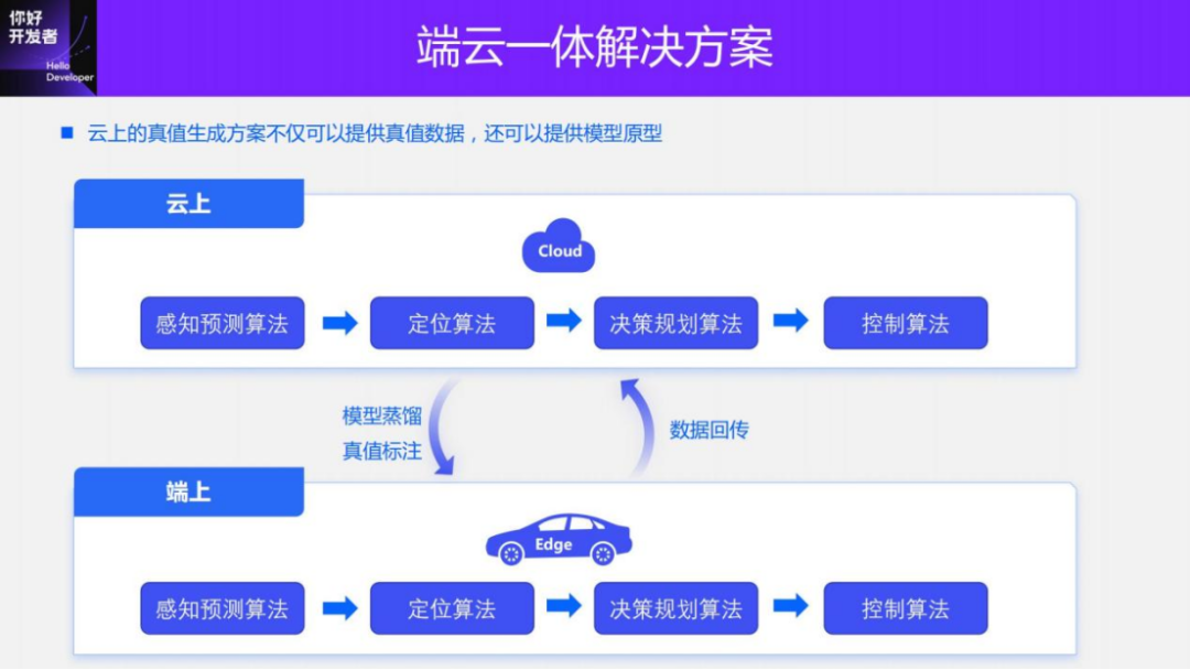
Going one step further, we can not only do simulation testing, but also integrate sensing solutions on the cloud and the car. The 4D Label true value generation solution is actually a complete intelligent driving solution including perception, positioning, decision-making and control in the cloud. As long as some geometric or rule-based things in the multi-mode and purely visual perception solutions introduced above are replaced with large models, it is actually a cloud-based smart driving solution.
A smart driving solution that integrates smart driving on the cloud and on the device can reduce maintenance costs. The cloud not only provides true value data to the on-device model, but also distills knowledge to the on-device model. The on-end model can explore some corner cases for iterating the cloud model.
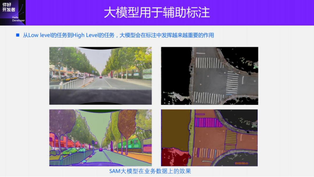
Another trend is that large models will play an increasingly important role in 4D Label annotation, from simple segmentation and detection tasks to more advanced annotation tasks such as behavior prediction, etc., in the form of knowledge transfer, to realize different tasks and different scenarios. knowledge sharing. These are some simple tests we did using business data. This is a large SAM segmentation model that can get some polygon annotations in 2D images. Compared with manual annotation, it can increase the annotation efficiency by 5 to 6 times. On the right is a texture mosaic image from the BEV perspective that we made using the SAM model directly to achieve the segmentation effect. Without pre-training, you can see that the segmentation effects of curbs and lane lines are already very good.
This is the main content I want to introduce today. Finally, to summarize:
1) 4D-Label for BEV’s true value system is a very important factor in model iteration efficiency and cost. Iteration efficiency and cost are the core competitiveness of AI products.
2) For 4D-Label, whether it is multi-modal labeling or purely visual labeling, high-precision and highly stable positioning and mapping are the basic modules of labeling. Whether it is for static annotation or end-to-end dynamic annotation, accurate pose is required.
3) Deployment of the end-to-end model on the end is a necessary step to achieve data closed loop. Some important post-processing tasks will move from the device to the cloud, becoming solutions for truth value annotation, and even becoming smart driving solutions for the cloud, which is the cloud-integrated architecture I just introduced.
4) Data simulation synthesis will be a very potential way to solve corner cases, and will definitely become a very important intelligent driving module infrastructure in the future.
This is the main content I want to introduce today. You are also welcome to pay attention to our future courses on autonomous driving. Thank you all.