Data Structures: Complexity Analysis

Find the solution to the problem : The algorithm needs to reliably find the correct solution to the problem within the specified input range.
Seeking the optimal solution : There may be multiple solutions to the same problem, and we hope to find an algorithm that is as efficient as possible.

In other words, on the premise that the problem can be solved, algorithm efficiency has become the main evaluation index to measure the quality of the algorithm, which includes the following two dimensions.

Time efficiency : How fast the algorithm runs.
Space efficiency : The amount of memory space occupied by the algorithm.

In short, our goal is to design data structures and algorithms that are "fast and economical" . It is crucial to effectively evaluate algorithm efficiency, because only in this way can we compare various algorithms to guide the algorithm design and optimization process.

There are two main methods of efficiency evaluation: actual testing and theoretical estimation.

1.1 Actual test

Suppose we now have an algorithm A and an algorithm B , both of which can solve the same problem, and now we need to compare the efficiency of these two algorithms. The most direct method is to find a computer, run these two algorithms, and monitor and record their running time and memory usage. This evaluation method can reflect the real situation, but it also has major limitations.

On the one hand, it is difficult to eliminate interference factors in the test environment . Hardware configuration will affect the performance of the algorithm. For example, in a certain computer, A the running time of the algorithm B is shorter than that of the algorithm; but in another computer with a different configuration, we may get the opposite test results. This means that we need to test on various machines and calculate the average efficiency, which is unrealistic.

On the other hand, rolling out full testing is very resource intensive . As the amount of input data changes, the algorithm will show different efficiencies. For example, when the amount of input data is small, A the running time of the algorithm B is less than that of the algorithm; when the amount of input data is large, the test results may be exactly the opposite. Therefore, in order to draw convincing conclusions, we need to test input data of various sizes, which requires a lot of computing resources.

1.2 Theoretical estimation

Since practical testing has major limitations, we can consider evaluating the efficiency of the algorithm through only some calculations. This estimation method is called "asymptotic complexity analysis", or "complexity analysis" for short.

Complexity analysis reflects the relationship between the time (space) resources required to run the algorithm and the size of the input data. It describes the increasing trend in time and space required for algorithm execution as the input data size increases . This definition is a bit confusing, and we can understand it by dividing it into three key points.

"Time and space resources" correspond to "time complexity" and "space complexity" respectively.
"As input data size increases" means that complexity reflects the relationship between the efficiency of the algorithm and the volume of input data.
"Growth trend of time and space" means that complexity analysis focuses not on the specific values of running time or occupied space, but on the "speed" of time or space growth.

Complexity analysis overcomes the shortcomings of actual testing methods , which is reflected in the following two aspects.

It is independent of the test environment and the analysis results are applicable to all running platforms.
It can reflect the algorithm efficiency under different data volumes, especially the algorithm performance under large data volumes.

Tip

If you're still confused about the concept of complexity, don't worry, we'll cover it in detail in subsequent chapters.

Complexity analysis provides us with a "ruler" to evaluate the efficiency of an algorithm, allowing us to measure the time and space resources required to execute an algorithm and compare the efficiency of different algorithms.

Complexity is a mathematical concept, which may be abstract and difficult for beginners to learn. From this perspective, complexity analysis may not be an appropriate first introduction. However, when we discuss the characteristics of a certain data structure or algorithm, it is difficult to avoid analyzing its running speed and space usage.

To sum up, it is recommended that you first establish a preliminary understanding of complexity analysis before learning about data structures and algorithms in depth , so that you can complete the complexity analysis of simple algorithms .

2 Iteration and recursion

In data structures and algorithms, it is very common to perform a certain task repeatedly, which is closely related to the complexity of the algorithm. To repeatedly perform a task, we usually use two basic program structures: iteration and recursion.

2.1 Iteration

"Iteration" is a control structure that repeatedly performs a task. In iteration, the program will repeatedly execute a certain code if certain conditions are met until the condition is no longer met.

1. for loop

for Loops are one of the most common forms of iteration and are suitable for use when the number of iterations is known in advance .

The following function for implements the sum 1+2+⋯+n based on a loop, and the summation result res is recorded using variables. It should be noted that range(a, b) the corresponding interval in Python is "closed on the left and open on the right", and the corresponding traversal range is a, a+1,...,b−1.

/* for 循环 */
int forLoop(int n) {
    int res = 0;
    // 循环求和 1, 2, ..., n-1, n
    for (int i = 1; i <= n; i++) {
        res += i;
    }
    return res;
}

Figure 2-1 shows the flow diagram of this summation function.

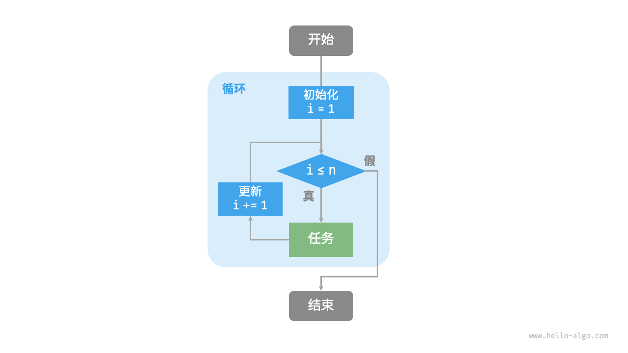
Figure 2-1 Flow chart of summation function

The number of operations of this summation function is proportional to the input data size n, or "linear". In fact, time complexity describes this "linear relationship" . Relevant content will be introduced in detail in the next section.

2. while loop

Similar to for loops, while loops are also a way to implement iteration. In while the loop, the program will first check the condition each round, and if the condition is true, it will continue to execute, otherwise it will end the loop.

Next, we use while a loop to implement the sum 1+2+⋯+�n.

/* while 循环 */
int whileLoop(int n) {
    int res = 0;
    int i = 1; // 初始化条件变量
    // 循环求和 1, 2, ..., n-1, n
    while (i <= n) {
        res += i;
        i++; // 更新条件变量
    }
    return res;
}

In while a loop, since the steps of initializing and updating condition variables are independent of the loop structure, it has for a higher degree of freedom than a loop .

For example, in the following code, the condition variable i is updated twice in each round. This situation is not convenient to for implement using a loop.

/* while 循环（两次更新） */
int whileLoopII(int n) {
    int res = 0;
    int i = 1; // 初始化条件变量
    // 循环求和 1, 4, ...
    while (i <= n) {
        res += i;
        // 更新条件变量
        i++;
        i *= 2;
    }
    return res;
}

In general, for the code for loops is more compact, while loops are more flexible , and both can implement iterative structures. The choice of which one to use should be based on the needs of the specific problem.

3. Nested loops

We can nest another loop structure within a loop structure, taking for loop as an example:

/* 双层 for 循环 */
char *nestedForLoop(int n) {
    // n * n 为对应点数量，"(i, j), " 对应字符串长最大为 6+10*2，加上最后一个空字符 \0 的额外空间
    int size = n * n * 26 + 1;
    char *res = malloc(size * sizeof(char));
    // 循环 i = 1, 2, ..., n-1, n
    for (int i = 1; i <= n; i++) {
        // 循环 j = 1, 2, ..., n-1, n
        for (int j = 1; j <= n; j++) {
            char tmp[26];
            snprintf(tmp, sizeof(tmp), "(%d, %d), ", i, j);
            strncat(res, tmp, size - strlen(res) - 1);
        }
    }
    return res;
}

Figure 2-2 shows the flow diagram of this nested loop.

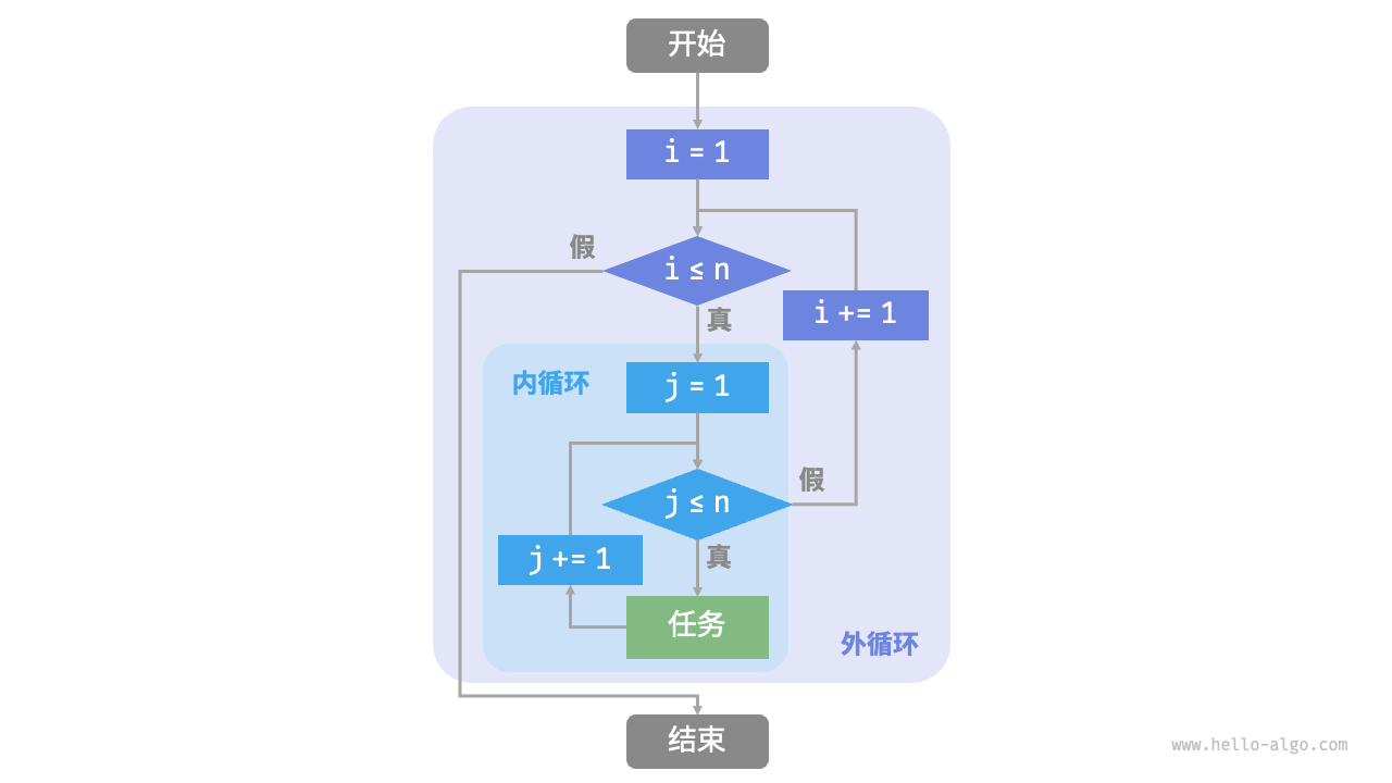
Figure 2-2 Flow chart of nested loop

In this case, the number of operations of the function is proportional to �2, or the algorithm running time is "squared" with the input data size �.

We can continue to add nested loops. Each nesting is a "dimension increase", which will increase the time complexity to "cubic relationship", "fourth power relationship", and so on.

2.2 Recursion

"Recursion" is an algorithmic strategy that solves problems by calling a function itself. It mainly consists of two stages.

Pass : The program calls itself deeper and deeper, usually passing in smaller or simplified parameters, until a "termination condition" is reached.
Return : After triggering the "termination condition", the program returns layer by layer starting from the deepest recursive function, and aggregates the results of each layer.

From an implementation perspective, recursive code mainly contains three elements.

Termination condition : used to determine when to switch from "delivery" to "return".
Recursive call : Corresponding to "recursive", the function calls itself, usually inputting smaller or simplified parameters.
Return result : Corresponds to "return", returning the results of the current recursive level to the previous level.

Observing the following code, we only need to call the function recur(n) to complete the calculation of 1+2+⋯+n:

/* 递归 */
int recur(int n) {
    // 终止条件
    if (n == 1)
        return 1;
    // 递：递归调用
    int res = recur(n - 1);
    // 归：返回结果
    return n + res;
}

Figure 2-3 shows the recursive process of this function.

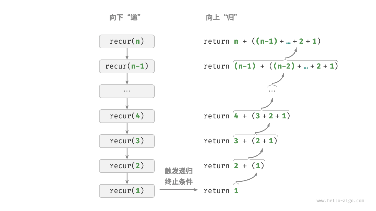
Figure 2-3 Recursive process of summation function

Although iteration and recursion can achieve the same results from a computational perspective, they represent two completely different paradigms for thinking and solving problems .

Iteration : Solving problems “from the bottom up.” Start with the most basic steps and then repeat or add up to them until the task is complete.
Recursion : Solving problems “from the top down”. Decompose the original problem into smaller sub-problems that have the same form as the original problem. Next, the sub-problem is continued to be decomposed into smaller sub-problems until it stops at the base case (the solution to the base case is known).

Taking the above summation function as an example, assume the problem f(n)=1+2+⋯+n.

Iteration : Simulate the summation process in a loop, traverse from 1 to �n, and perform the summation operation in each round to obtain f(n).
Recursion : Decompose the problem into sub-problems f(n)=n+f(n−1), and continue to decompose (recursively) until the basic case f(1)=1.

1. Call stack

Each time a recursive function calls itself, the system allocates memory for the newly opened function to store local variables, calling addresses and other information. This will have two consequences.

The context data of the function is stored in a memory area called the "stack frame space" and will not be released until the function returns. Therefore, recursion usually consumes more memory space than iteration .
Calling functions recursively incurs additional overhead. Therefore recursion is usually less time efficient than looping .

As shown in Figure 2-4, before the termination condition is triggered, there are n unreturning recursive functions at the same time, and the recursion depth is n .

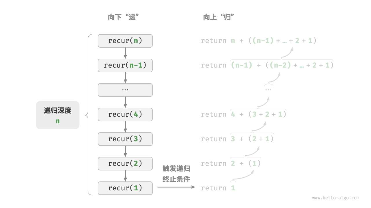
Figure 2-4 Recursive call depth

In practice, the recursion depth allowed by a programming language is usually limited, and excessively deep recursion may result in a stack overflow error.

2. Tail recursion

Interestingly, if a function makes a recursive call as the last step before returning , the function can be optimized by the compiler or interpreter to be as space-efficient as iteration. This situation is called "tail recursion".

Ordinary recursion : When the function returns to the function at the upper level, it needs to continue executing the code, so the system needs to save the context of the previous level call.
Tail recursion : The recursive call is the last operation before the function returns, which means that after the function returns to the previous level, there is no need to continue to perform other operations, so the system does not need to save the context of the previous level function.

Taking the calculation of 1+2+⋯+n as an example, we can set the result variable res as a function parameter to achieve tail recursion.

/* 尾递归 */
int tailRecur(int n, int res) {
    // 终止条件
    if (n == 0)
        return res;
    // 尾递归调用
    return tailRecur(n - 1, res + n);
}

The execution process of tail recursion is shown in Figure 2-5. Comparing ordinary recursion and tail recursion, the execution points of the sum operation are different.

Ordinary recursion : The summation operation is performed during the "return" process, and the summation operation must be performed again after each layer returns.
Tail recursion : The summation operation is performed in the "recursive" process, and the "return" process only needs to return layer by layer.

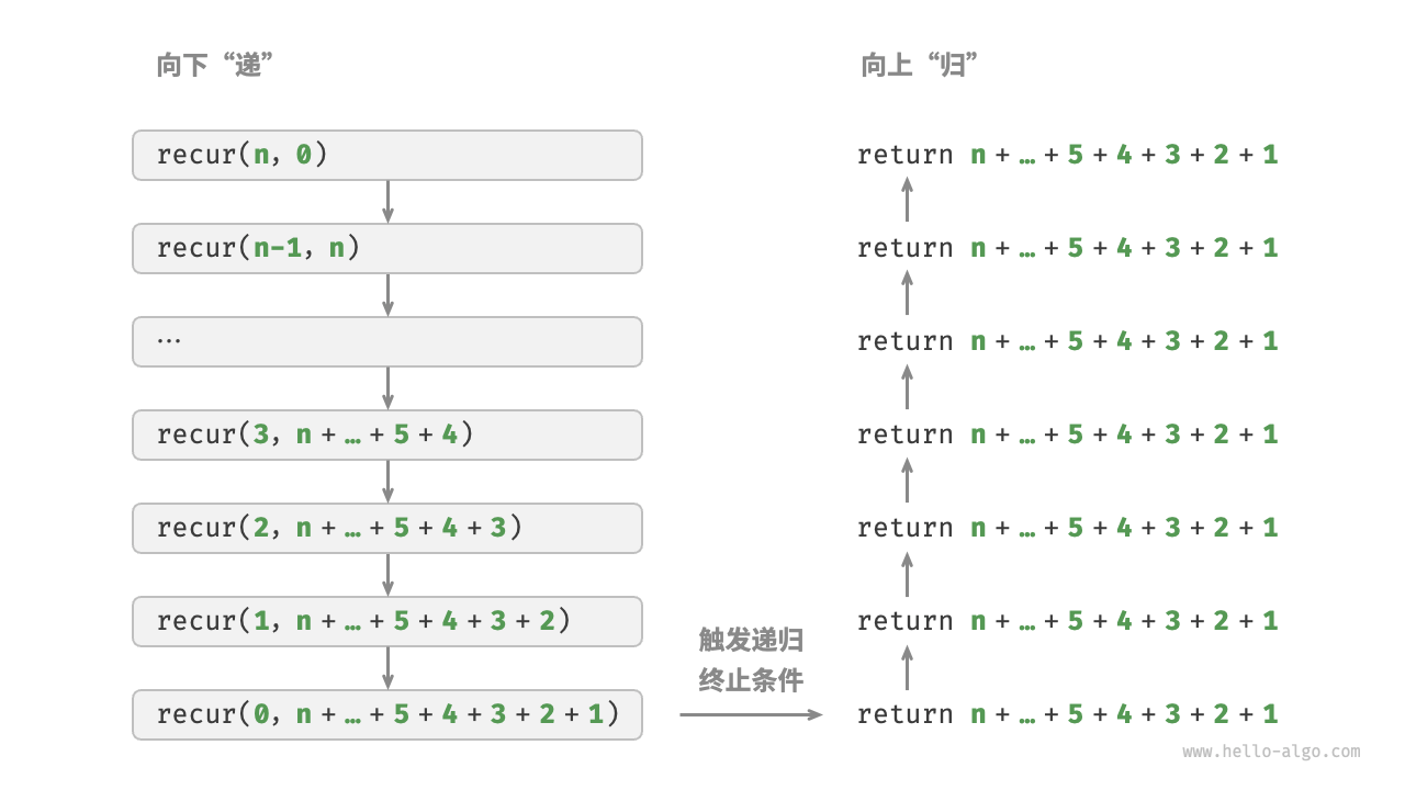
Figure 2-5 Tail recursive process

Tip

Note that many compilers or interpreters do not support tail recursion optimization. For example, Python does not support tail recursive optimization by default, so even if the function is tail recursive, you may still encounter stack overflow problems.

3. Recursive tree

When dealing with algorithmic problems related to "divide and conquer", recursion is often more intuitive and the code is more readable than iteration. Take the "Fibonacci Sequence" as an example.

Question

Given a Fibonacci sequence 0,1,1,2,3,5,8,13,… , find the �th number in the sequence.

Assuming that the nth number in the Fibonacci sequence is f(n), it is easy to draw two conclusions.

The first two numbers in the sequence are f(1)=0 and f(2)=1.
Each number in the sequence is the sum of the previous two numbers, that is, f(n)=f(n−1)+f(n−2).

Make recursive calls according to the recursion relationship, and use the first two numbers as the termination condition to write recursive code. Call fib(n) to get the nth number of the Fibonacci sequence.

/* 斐波那契数列：递归 */
int fib(int n) {
    // 终止条件 f(1) = 0, f(2) = 1
    if (n == 1 || n == 2)
        return n - 1;
    // 递归调用 f(n) = f(n-1) + f(n-2)
    int res = fib(n - 1) + fib(n - 2);
    // 返回结果 f(n)
    return res;
}

Observing the above code, we are calling two functions recursively within the function, which means that two call branches are generated from one call . As shown in Figure 2-6, this continuous recursive call will eventually produce a "recursion tree" with n levels.

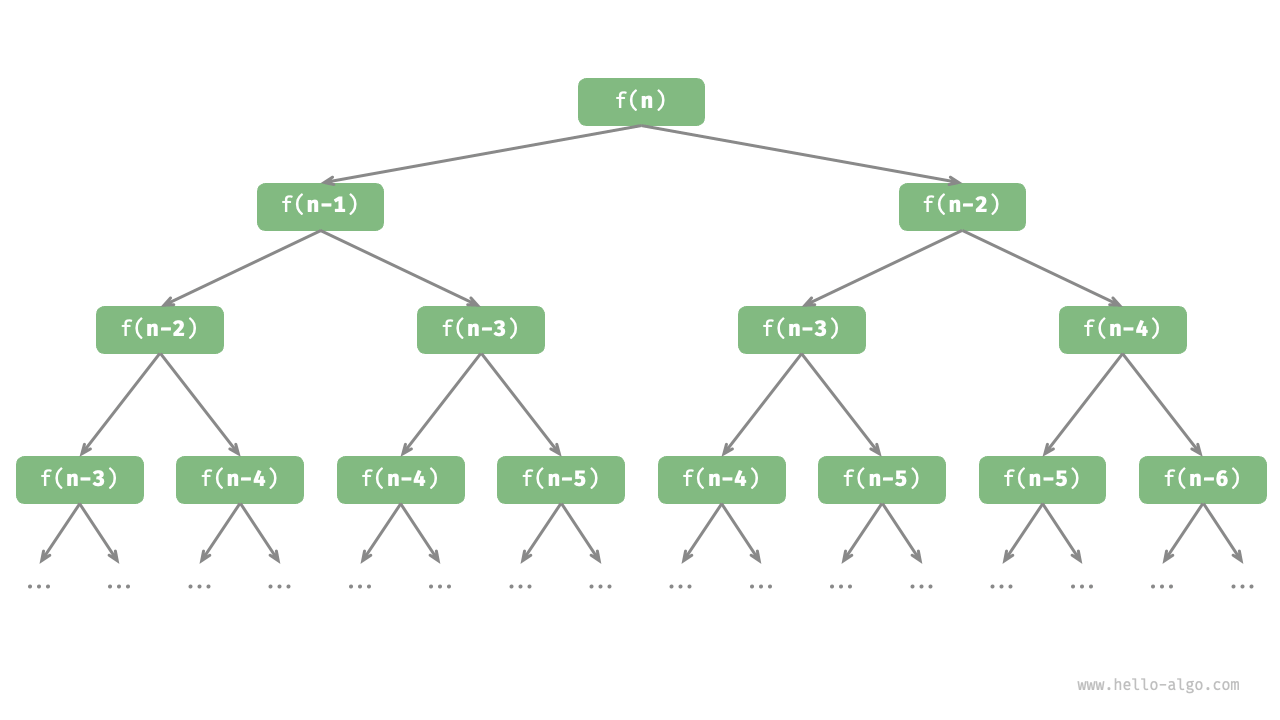
Figure 2-6 Recursion tree of Fibonacci sequence

In essence, recursion embodies the thinking paradigm of "decomposing the problem into smaller sub-problems". This divide-and-conquer strategy is crucial.

From an algorithmic perspective, many important algorithmic strategies such as search, sorting, backtracking, divide and conquer, and dynamic programming directly or indirectly apply this way of thinking.
From a data structure perspective, recursion is naturally suitable for dealing with problems related to linked lists, trees and graphs, because they are very suitable for analysis using divide and conquer thinking.

2.3 Comparison between the two

To summarize the above, as shown in Table 2-1, iteration and recursion differ in implementation, performance, and applicability.

Table 2-1 Comparison of characteristics of iteration and recursion

	Iterate	recursion
Method to realize	Loop structure	function calls itself
time efficiency	Usually more efficient, no function call overhead	Each function call incurs overhead
memory usage	Usually uses a fixed size memory space	Cumulative function calls may use a large amount of stack frame space
Applicable issues	Suitable for simple loop tasks, the code is intuitive and readable	Suitable for sub-problem decomposition, such as trees, graphs, divide and conquer, backtracking, etc., the code structure is concise and clear

Tip

If you find it difficult to understand the following content, you can review it after reading the "Stack" chapter.

So, what is the intrinsic connection between iteration and recursion? Taking the above recursive function as an example, the summation operation is performed in the "return" phase of the recursion. This means that the function called initially is actually the last to complete its sum operation. This working mechanism is similar to the "first in, last out" principle of the stack .

In fact, recursive terms such as "call stack" and "stack frame space" already imply the close relationship between recursion and the stack.

Pass : When a function is called, the system will allocate a new stack frame for the function on the "call stack" to store the function's local variables, parameters, return address and other data.
Return : When the function completes execution and returns, the corresponding stack frame will be removed from the "call stack" and the execution environment of the previous function will be restored.

Therefore, we can use an explicit stack to simulate the behavior of a call stack , thus converting recursion into iterative form:

[class]{}-[func]{forLoopRecur}

Observe the above code, when the recursion is converted into iteration, the code becomes more complex. Although iteration and recursion can be converted into each other in many cases, it is not always worth doing so for two reasons.

The transformed code may be more difficult to understand and less readable.
For some complex problems, simulating the behavior of the system call stack can be very difficult.

In summary, the choice between iteration and recursion depends on the nature of the particular problem . In programming practice, it is crucial to weigh the pros and cons of both and choose the appropriate method based on the situation.

3 Time complexity

Running time can intuitively and accurately reflect the efficiency of the algorithm. If we want to accurately estimate the running time of a piece of code, how should we do it?

Determine the running platform , including hardware configuration, programming language, system environment, etc. These factors will affect the running efficiency of the code.
Evaluate the running time required for various calculation operations , such as addition operations + requiring 1 ns, multiplication operations * requiring 10 ns, printing operations print() requiring 5 ns, etc.
All calculation operations in the code are counted , and the execution time of all operations is summed to obtain the running time.

For example, in the following code, the input data size is n:

// 在某运行平台下
void algorithm(int n) {
    int a = 2;  // 1 ns
    a = a + 1;  // 1 ns
    a = a * 2;  // 10 ns
    // 循环 n 次
    for (int i = 0; i < n; i++) {   // 1 ns ，每轮都要执行 i++
        printf("%d", 0);            // 5 ns
    }
}

According to the above method, the algorithm running time can be obtained as 6n+12 ns:

1+1+10+(1+5)×n=6n+12

But in practice, the running time of statistical algorithms is neither reasonable nor realistic . First of all, we do not want to tie the estimated time to the running platform, because the algorithm needs to run on a variety of different platforms. Secondly, it is difficult to know the running time of each operation, which makes the estimation process extremely difficult.

3.1 Statistical time growth trend

Time complexity analysis counts not the algorithm running time, but the growth trend of the algorithm running time as the amount of data increases .

The concept of "time growth trend" is relatively abstract. Let's understand it through an example. Assume that the input data size is n, given three algorithm functions A, B and C :

// 算法 A 的时间复杂度：常数阶
void algorithm_A(int n) {
    printf("%d", 0);
}
// 算法 B 的时间复杂度：线性阶
void algorithm_B(int n) {
    for (int i = 0; i < n; i++) {
        printf("%d", 0);
    }
}
// 算法 C 的时间复杂度：常数阶
void algorithm_C(int n) {
    for (int i = 0; i < 1000000; i++) {
        printf("%d", 0);
    }
}

Figure 2-7 shows the time complexity of the above three algorithm functions.

The algorithm A has only one printing operation, and the running time of the algorithm does not increase as n increases. We call the time complexity of this algorithm "constant order".
The printing operation in the algorithm B needs to be looped n times, and the algorithm running time increases linearly as n increases. The time complexity of this algorithm is called "linear order".
C The printing operation in the algorithm needs to loop 1000000 times. Although the running time is very long, it has nothing to do with the input data size n. Therefore C , the time complexity A is the same as that of "constant order".

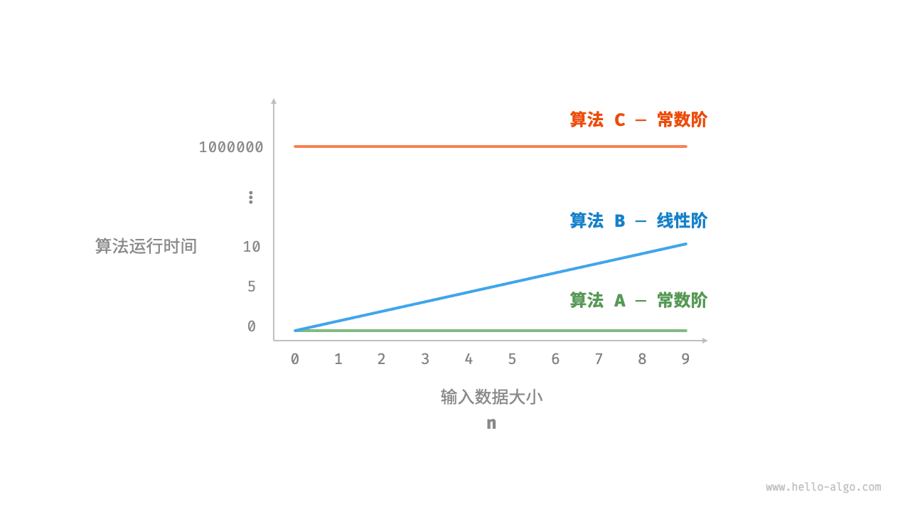
Figure 2-7 Time growth trend of algorithms A, B and C

Compared with directly counting algorithm running time, what are the characteristics of time complexity analysis?

Time complexity can effectively evaluate algorithm efficiency . For example, the running time of the algorithm increases linearly, is slower B than the algorithm when n>1 , and is slower than the algorithm when n>1000000. In fact, as long as the input data size n is large enough, an algorithm with a "constant order" complexity must be better than a "linear order" algorithm. This is exactly what the time growth trend expresses.AC
The time complexity calculation method is simpler . Apparently, neither the running platform nor the type of computational operations are related to the increasing trend of algorithm running time. Therefore, in time complexity analysis, we can simply regard the execution time of all calculation operations as the same "unit time", thereby simplifying "the statistics of the running time of calculation operations" to "the statistics of the number of calculation operations", In this way, the difficulty of estimation is greatly reduced.
There are also certain limitations in time complexity . For example, although the time complexity of the algorithms A A and A is the same, the actual running times vary significantly. CSimilarly, although B the time complexity ratio of the algorithm C is high , the algorithm B is significantly better than the algorithm when the input data size n is small C . In these cases, it is difficult for us to judge the efficiency of an algorithm based on time complexity alone. Of course, despite the above problems, complexity analysis is still the most effective and commonly used method to judge the efficiency of an algorithm.

3.2 Function asymptotic upper bound

Given a function with input size n:

void algorithm(int n) {
    int a = 1;  // +1
    a = a + 1;  // +1
    a = a * 2;  // +1
    // 循环 n 次
    for (int i = 0; i < n; i++) {   // +1（每轮都执行 i ++）
        printf("%d", 0);            // +1
    }
}

Assume that the number of operations of the algorithm is a function of the input data size n, denoted as T(n), then the number of operations of the above function is:

T(n)=3+2n

T(n) is a linear function, which means that the growth trend of its running time is linear, so its time complexity is linear order.

We record the time complexity of linear order as O(n). This mathematical symbol is called "big-O notation", which represents the "asymptotic upper bound" of the function T(n).

Time complexity analysis is essentially the calculation of the asymptotic upper bound of the "operation number function T(n)", which has a clear mathematical definition.

As shown in Figure 2-8, calculating the asymptotic upper bound is to find a function f(n) such that when n tends to infinity, T(n) and f(n) are at the same growth level, with only one constant difference. Multiples of c.

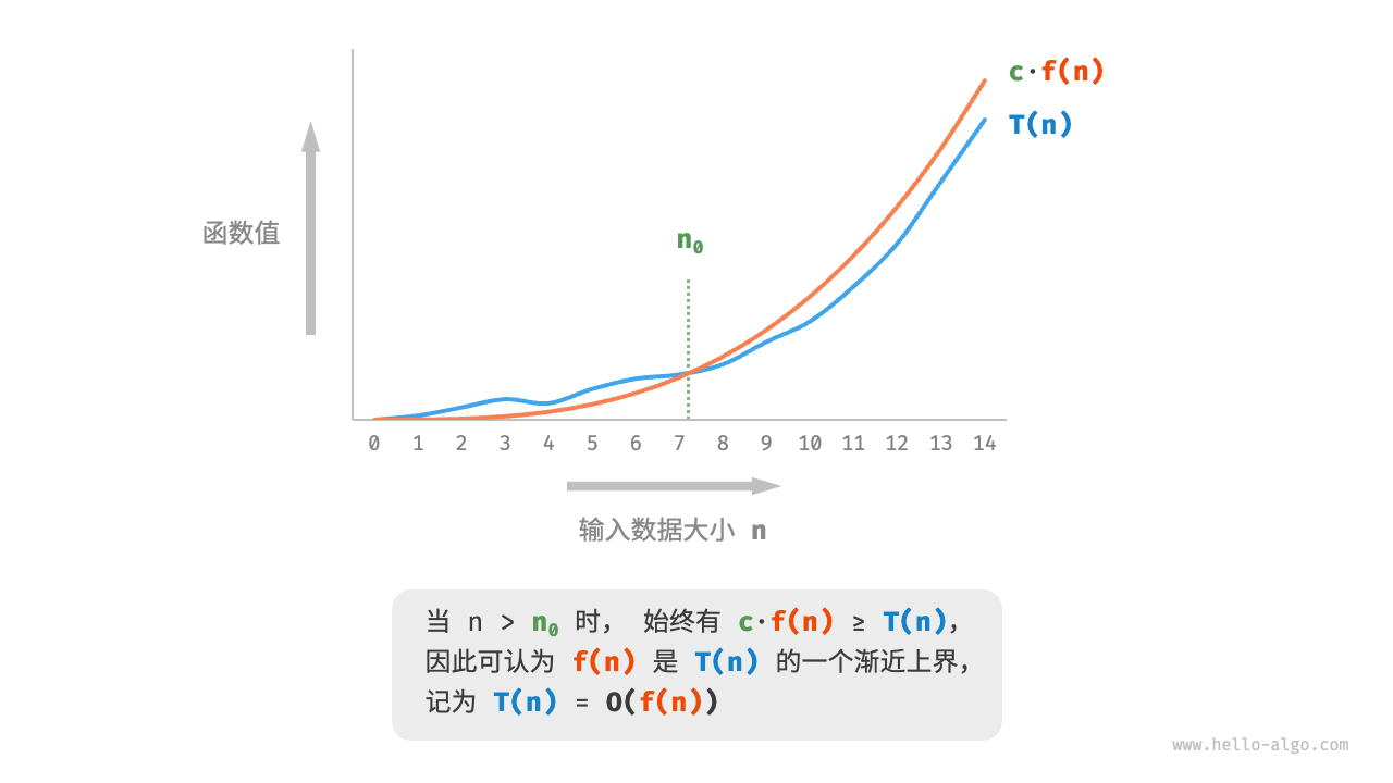
Figure 2-8 Asymptotic upper bound of function

3.3 Calculation method

Asymptotic upper bounds are a bit mathematical, so don't worry if you don't feel you fully understand them. Because in actual use, we only need to master the calculation method, and the mathematical meaning can be gradually understood.

1. Step 1: Count the number of operations

For the code, just calculate it line by line from top to bottom. However, since the constant term c in the above c⋅f(n) can take any size, the various coefficients and constant terms in the operation number f(n) can be ignored . Based on this principle, the following counting simplification techniques can be summarized.

Ignore the constant terms in f(n) . Because they are independent of n, they have no impact on the time complexity.
Omit all coefficients . For example, looping 2n times, 5n+1 times, etc. can be simplified and recorded as n times, because the coefficients in front of n have no impact on the time complexity.
Use multiplication when nesting loops . The total number of operations is equal to the product of the number of operations in the outer loop and the inner loop. Each loop can still apply the techniques at point 1 1. and point 1 respectively.2.

Given a function, we can count the number of operations using the above techniques.

void algorithm(int n) {
    int a = 1;  // +0（技巧 1）
    a = a + n;  // +0（技巧 1）
    // +n（技巧 2）
    for (int i = 0; i < 5 * n + 1; i++) {
        printf("%d", 0);
    }
    // +n*n（技巧 3）
    for (int i = 0; i < 2 * n; i++) {
        for (int j = 0; j < n + 1; j++) {
            printf("%d", 0);
        }
    }
}

2. Step 2: Determine the asymptotic upper bound

The time complexity is determined by the highest order term in the polynomial T(n) . This is because as n approaches infinity, the highest-order term will play a dominant role, and the influence of other terms can be ignored.

Table 2-2 shows some examples, some of which are exaggerated to emphasize the conclusion that the coefficient cannot shake the order. As n goes to infinity, these constants become insignificant.

Table 2-2 Time complexity corresponding to different number of operations

Number of operations	time complexity
100000	O(1)
3n+2	O(n)
2n2+3n+2	O(n2)
n3+10000n2	O(n3)
2n+10000n10000	n(2n)

3.4 Common types

Assume the input data size is n, and the common time complexity types are shown in Figure 2-9 (arranged from low to high).

Constant order < logarithmic order < linear order < linear logarithmic order < square order < exponential order < factorial order

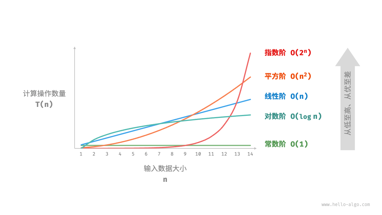
Figure 2-9 Common time complexity types

1. Constant order O(1)

The number of constant-order operations has nothing to do with the input data size n, that is, it does not change with the change of n.

In the following function, although the number of operations size may be large, the time complexity is still O(1) since it is independent of the input data size n:

/* 常数阶 */
int constant(int n) {
    int count = 0;
    int size = 100000;
    int i = 0;
    for (int i = 0; i < size; i++) {
        count++;
    }
    return count;
}

2. Linear order O(n)

The number of linear-order operations grows linearly with the input data size n. Linear orders usually occur in single-level loops:

/* 线性阶 */
int linear(int n) {
    int count = 0;
    for (int i = 0; i < n; i++) {
        count++;
    }
    return count;
}

The time complexity of traversing arrays and linked lists is O(n), where n is the length of the array or linked list:

/* 线性阶（遍历数组） */
int arrayTraversal(int *nums, int n) {
    int count = 0;
    // 循环次数与数组长度成正比
    for (int i = 0; i < n; i++) {
        count++;
    }
    return count;
}

It is worth noting that the input data size n needs to be specifically determined according to the type of input data .

3. Square order O(n2)

The number of square-order operations grows quadratically with the input data size n. Square order usually occurs in nested loops, where both the outer and inner loops are O(n), so the total is O(n2):

/* 平方阶 */
int quadratic(int n) {
    int count = 0;
    // 循环次数与数组长度成平方关系
    for (int i = 0; i < n; i++) {
        for (int j = 0; j < n; j++) {
            count++;
        }
    }
    return count;
}

Figure 2-10 compares the three time complexities of constant order, linear order and square order.

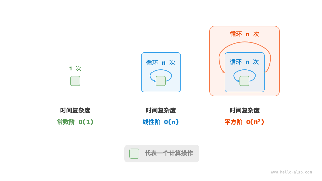
Figure 2-10 Time complexity of constant order, linear order and square order

Taking bubble sorting as an example, the outer loop is executed n−1 times, and the inner loop is executed n−1, n−2,...,2,1 times, with an average of n/2 times, so the time complexity is n(( n−1)n/2)=O(n2) .

/* 平方阶（冒泡排序） */
int bubbleSort(int *nums, int n) {
    int count = 0; // 计数器
    // 外循环：未排序区间为 [0, i]
    for (int i = n - 1; i > 0; i--) {
        // 内循环：将未排序区间 [0, i] 中的最大元素交换至该区间的最右端
        for (int j = 0; j < i; j++) {
            if (nums[j] > nums[j + 1]) {
                // 交换 nums[j] 与 nums[j + 1]
                int tmp = nums[j];
                nums[j] = nums[j + 1];
                nums[j + 1] = tmp;
                count += 3; // 元素交换包含 3 个单元操作
            }
        }
    }
    return count;
}

4. Exponential order O(2n)

Biological "cell division" is a typical example of exponential growth: the initial state is 1 cell, after one round of division it becomes 2, after two rounds of division it becomes 4, and so on, after n rounds of division there are 2n cells.

Figure 2-11 and the following code simulate the process of cell division, with a time complexity of O(2n).

/* 指数阶（循环实现） */
int exponential(int n) {
    int count = 0;
    int bas = 1;
    // 细胞每轮一分为二，形成数列 1, 2, 4, 8, ..., 2^(n-1)
    for (int i = 0; i < n; i++) {
        for (int j = 0; j < bas; j++) {
            count++;
        }
        bas *= 2;
    }
    // count = 1 + 2 + 4 + 8 + .. + 2^(n-1) = 2^n - 1
    return count;
}

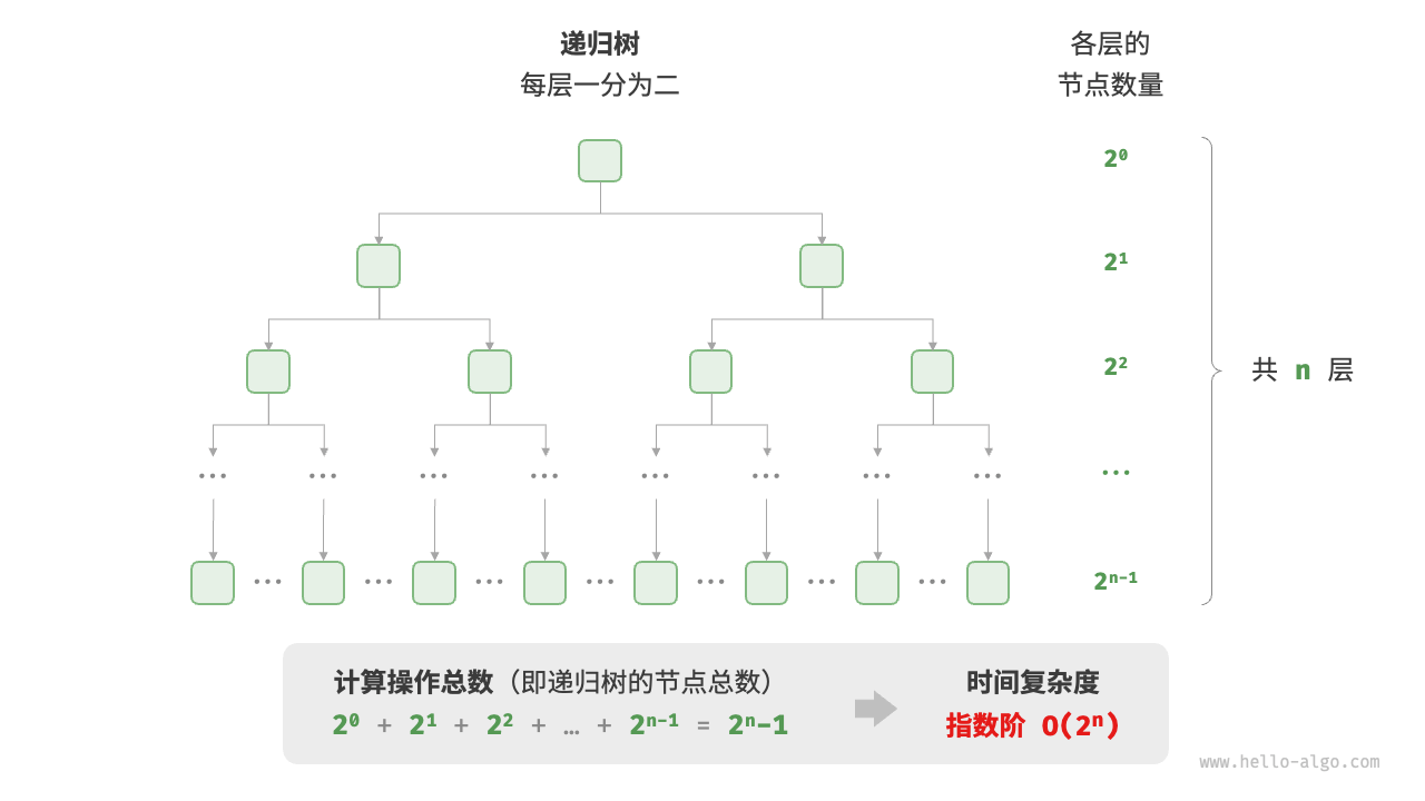
Figure 2-11 Exponential time complexity

In actual algorithms, exponential orders often appear in recursive functions. For example, in the following code, it recursively splits in two and stops after n splits:

/* 指数阶（递归实现） */
int expRecur(int n) {
    if (n == 1)
        return 1;
    return expRecur(n - 1) + expRecur(n - 1) + 1;
}

Exponential growth is very rapid and is common in exhaustive methods (brute force search, backtracking, etc.). For problems with large data sizes, exponential order is unacceptable and usually requires the use of dynamic programming or greedy algorithms to solve.

5. Logarithmic order O(log⁡n)

In contrast to the exponential order, the logarithmic order reflects a "halving each round" situation. Suppose the input data size is �. Since each round is reduced to half, the number of loops is log2⁡n, which is the inverse function of 2n.

Figure 2-12 and the following code simulate the process of "reducing each round to half". The time complexity is O(log2⁡n), abbreviated as O(log⁡n).

/* 对数阶（循环实现） */
int logarithmic(float n) {
    int count = 0;
    while (n > 1) {
        n = n / 2;
        count++;
    }
    return count;
}

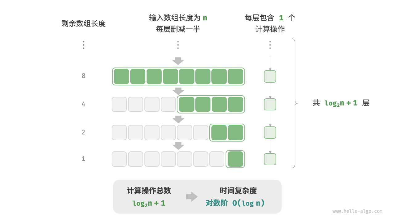
Figure 2-12 Logarithmic time complexity

Similar to the exponential order, the logarithmic order often appears in recursive functions. The following code forms a recursive tree of height log2⁡n:

/* 对数阶（递归实现） */
int logRecur(float n) {
    if (n <= 1)
        return 0;
    return logRecur(n / 2) + 1;
}

The logarithmic order often appears in algorithms based on the divide-and-conquer strategy, embodying the algorithmic ideas of “dividing one into many” and “simplifying complexity.” It grows slowly and is second only to the ideal time complexity of constant order.

6. Linear logarithmic order O(nlog⁡n)

Linear logarithmic order often appears in nested loops, and the time complexity of the two levels of loops is O(log⁡n) and O(n) respectively. The relevant code is as follows:

/* 线性对数阶 */
int linearLogRecur(float n) {
    if (n <= 1)
        return 1;
    int count = linearLogRecur(n / 2) + linearLogRecur(n / 2);
    for (int i = 0; i < n; i++) {
        count++;
    }
    return count;
}

Figure 2-13 shows how the linear logarithmic order is generated. The total number of operations at each level of the binary tree is n, and the tree has a total of log2⁡n+1 levels, so the time complexity is O(nlog⁡n).

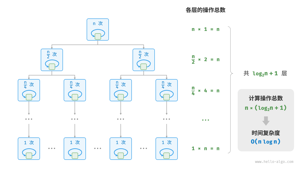
Figure 2-13 Time complexity of linear logarithmic order

The time complexity of mainstream sorting algorithms is usually O(nlog⁡n), such as quick sort, merge sort, heap sort, etc.

7. Factorial O(n!)

The factorial order corresponds to the "total permutation" problem in mathematics. Given n non-repeating elements, find all possible arrangements and the number of them

Factorial is usually implemented using recursion. As shown in Figure 2-14 and the following code, the first layer splits n pieces, the second layer splits n-1 pieces, and so on, until the nth layer splits:

/* 阶乘阶（递归实现） */
int factorialRecur(int n) {
    if (n == 0)
        return 1;
    int count = 0;
    for (int i = 0; i < n; i++) {
        count += factorialRecur(n - 1);
    }
    return count;
}

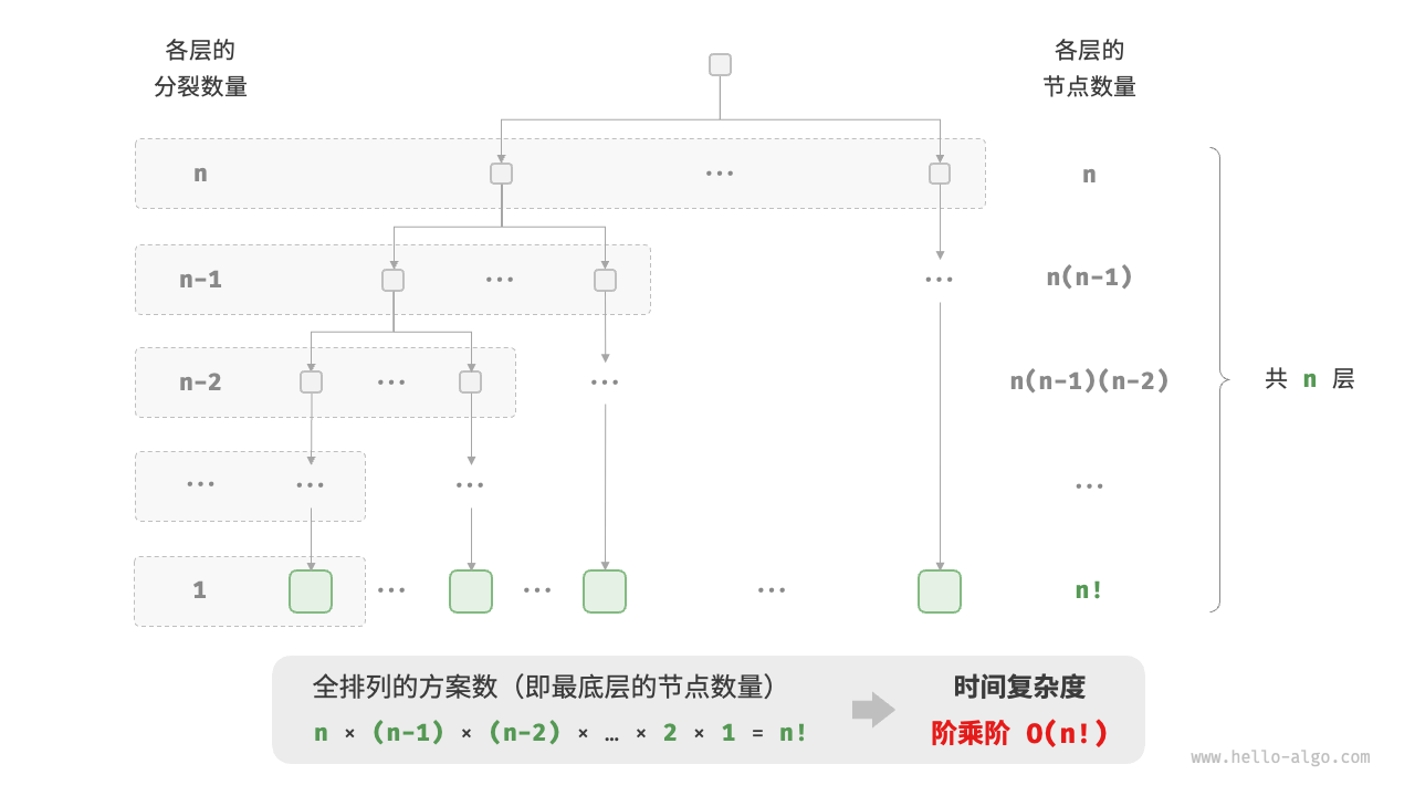
Figure 2-14 Time complexity of factorial factor

Please note that because there is always n!>2n when n≥4, the factorial order grows faster than the exponential order, which is also unacceptable when n is large.

3.5 Worst, best, and average time complexity

The time efficiency of an algorithm is often not fixed, but is related to the distribution of input data . Assume that an array of length � is input nums , which nums consists of numbers from 1 to n. Each number appears only once; but the order of the elements is randomly shuffled, and the task goal is to return the index of element 1. We can draw the following conclusions.

When nums = [?, ?, ..., 1] , that is, when the last element is 1, the array needs to be completely traversed, reaching the worst time complexity of O(n) .
When nums = [1, ?, ?, ...] , that is, when the first element is 1, no matter how long the array is, there is no need to continue traversing, and the optimal time complexity Ω(1) is achieved .

The "worst time complexity" corresponds to the asymptotic upper bound of the function, expressed in big O notation. Correspondingly, the "optimal time complexity" corresponds to the asymptotic lower bound of the function, represented by Ω notation:

/* 生成一个数组，元素为 { 1, 2, ..., n }，顺序被打乱 */
int *randomNumbers(int n) {
    // 分配堆区内存（创建一维可变长数组：数组中元素数量为 n ，元素类型为 int ）
    int *nums = (int *)malloc(n * sizeof(int));
    // 生成数组 nums = { 1, 2, 3, ..., n }
    for (int i = 0; i < n; i++) {
        nums[i] = i + 1;
    }
    // 随机打乱数组元素
    for (int i = n - 1; i > 0; i--) {
        int j = rand() % (i + 1);
        int temp = nums[i];
        nums[i] = nums[j];
        nums[j] = temp;
    }
    return nums;
}

/* 查找数组 nums 中数字 1 所在索引 */
int findOne(int *nums, int n) {
    for (int i = 0; i < n; i++) {
        // 当元素 1 在数组头部时，达到最佳时间复杂度 O(1)
        // 当元素 1 在数组尾部时，达到最差时间复杂度 O(n)
        if (nums[i] == 1)
            return i;
    }
    return -1;
}

It is worth mentioning that we rarely use the optimal time complexity in practice, because it can usually only be achieved with a small probability, which may be misleading. The worst time complexity is more practical because it gives an efficiency and safety value so that we can use the algorithm with confidence.

As can be seen from the above examples, the worst or best time complexity only appears in "special data distribution". The probability of occurrence of these situations may be very small and cannot truly reflect the efficiency of the algorithm. In contrast, the average time complexity can reflect the operating efficiency of the algorithm under random input data , represented by the notation Θ.

For some algorithms, we can simply extrapolate the average situation under a random data distribution. For example, in the above example, since the input array is scrambled, the probability of element 1 appearing at any index is equal, then the average number of loops of the algorithm is half of the array length n/2, and the average time complexity is Θ(n /2)=Θ(n) .

But for more complex algorithms, it is often difficult to calculate the average time complexity because it is difficult to analyze the overall mathematical expectation under the data distribution. In this case, we usually use the worst time complexity as the criterion for algorithm efficiency.

Why is the Θ symbol rarely seen?

Perhaps because the O symbol is so catchy, we often use it to represent average time complexity. But in a strict sense, this approach is not standardized. In this book and other materials, if you encounter expressions like "average time complexity O(n)", please understand it directly as Θ(n).

4 Space complexity

"Space complexity" is used to measure the growth trend of the memory space occupied by the algorithm as the amount of data increases. The concept is very similar to time complexity, just replace "running time" with "memory space occupied".

4.1 Algorithm-related space

The memory space used by the algorithm during operation mainly includes the following types.

Input space : used to store input data for the algorithm.
Temporary storage space : used to store variables, objects, function context and other data during the running process of the algorithm.
Output space : used to store the output data of the algorithm.

Generally speaking, the statistical range of space complexity is "temporary space" plus "output space".

The staging space can be further divided into three parts.

Temporary data : used to save various constants, variables, objects, etc. during the operation of the algorithm.
Stack frame space : used to save context data of calling functions. The system creates a stack frame on the top of the stack every time a function is called. After the function returns, the stack frame space is released.
Instruction space : used to save compiled program instructions, which is usually ignored in actual statistics.

When analyzing the space complexity of a program, we usually count three parts: temporary data, stack frame space and output data .

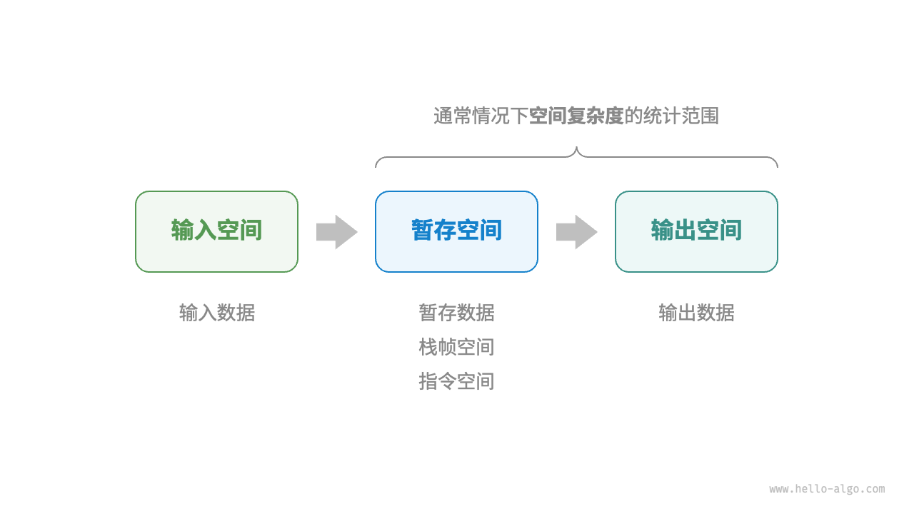
Figure 2-15 Correlation space used by the algorithm

/* 函数 */
int func() {
    // 执行某些操作...
    return 0;
}

int algorithm(int n) { // 输入数据
    const int a = 0;   // 暂存数据（常量）
    int b = 0;         // 暂存数据（变量）
    int c = func();    // 栈帧空间（调用函数）
    return a + b + c;  // 输出数据
}

4.2 Calculation method

The calculation method of space complexity is roughly the same as that of time complexity. You only need to change the statistical object from "number of operations" to "used space size".

Unlike time complexity, we usually only focus on the worst space complexity . This is because memory space is a hard requirement and we must ensure that sufficient memory space is reserved for all input data.

Observing the following code, the "worst" in the worst space complexity has two meanings.

Based on the worst input data : when n<10, the space complexity is O(1); but when n>10, the initialized array nums occupies O(n) space; therefore, the worst space complexity is O(n ).
Based on the peak memory during algorithm running : for example, the program occupies O(1) space before executing the last line; when initializing the array nums , the program occupies O(n) space; therefore, the worst space complexity is O(n) .

void algorithm(int n) {
    int a = 0;               // O(1)
    int b[10000];            // O(1)
    if (n > 10)
        int nums[n] = {0};   // O(n)
}

In recursive functions, you need to pay attention to stack frame space statistics . For example in the following code:

The function loop() is called n times in the loop function() , and the stack frame space is returned and released in each round function() , so the space complexity is still O(1).
recur() There will be n unreturned recursive functions at the same time during operation recur() , thus occupying O(n) stack frame space.

int func() {
    // 执行某些操作
    return 0;
}
/* 循环 O(1) */
void loop(int n) {
    for (int i = 0; i < n; i++) {
        func();
    }
}
/* 递归 O(n) */
void recur(int n) {
    if (n == 1) return;
    return recur(n - 1);
}

4.3 Common types

Assuming the input data size is n, Figure 2-16 shows common space complexity types (arranged from low to high).

Constant order < logarithmic order < linear order < square order < exponential order

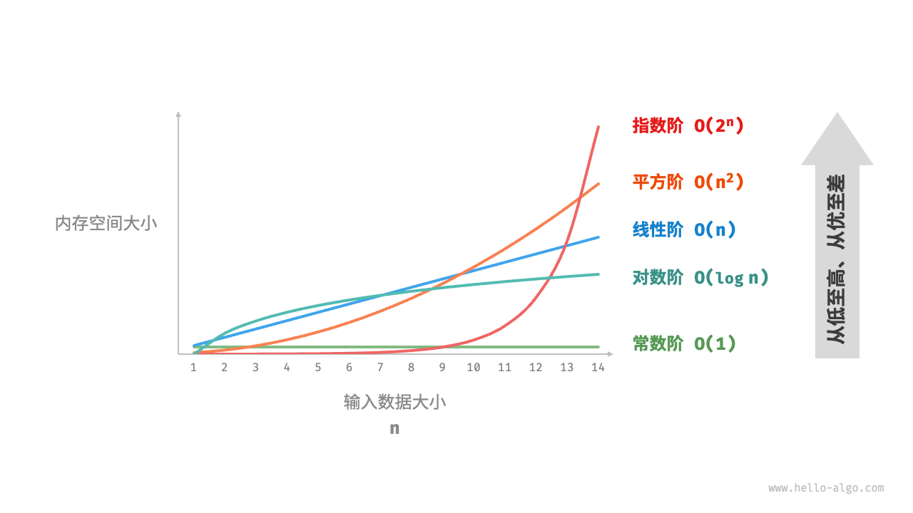
Figure 2-16 Common types of space complexity

1. Constant order O(1)

Constant order is common in constants, variables, and objects whose number has nothing to do with the input data size n.

It should be noted that the memory occupied by initializing variables or calling functions in a loop will be released after entering the next loop, so the occupied space will not accumulate, and the space complexity is still O(1):

/* 函数 */
int func() {
    // 执行某些操作
    return 0;
}

/* 常数阶 */
void constant(int n) {
    // 常量、变量、对象占用 O(1) 空间
    const int a = 0;
    int b = 0;
    int nums[1000];
    ListNode *node = newListNode(0);
    free(node);
    // 循环中的变量占用 O(1) 空间
    for (int i = 0; i < n; i++) {
        int c = 0;
    }
    // 循环中的函数占用 O(1) 空间
    for (int i = 0; i < n; i++) {
        func();
    }
}

2. Linear order O(n)

Linear order is common in arrays, linked lists, stacks, queues, etc. where the number of elements is proportional to n:

/* 哈希表 */
struct hashTable {
    int key;
    int val;
    UT_hash_handle hh; // 基于 uthash.h 实现
};

typedef struct hashTable hashTable;

/* 线性阶 */
void linear(int n) {
    // 长度为 n 的数组占用 O(n) 空间
    int *nums = malloc(sizeof(int) * n);
    free(nums);

    // 长度为 n 的列表占用 O(n) 空间
    ListNode **nodes = malloc(sizeof(ListNode *) * n);
    for (int i = 0; i < n; i++) {
        nodes[i] = newListNode(i);
    }
    // 内存释放
    for (int i = 0; i < n; i++) {
        free(nodes[i]);
    }
    free(nodes);

    // 长度为 n 的哈希表占用 O(n) 空间
    hashTable *h = NULL;
    for (int i = 0; i < n; i++) {
        hashTable *tmp = malloc(sizeof(hashTable));
        tmp->key = i;
        tmp->val = i;
        HASH_ADD_INT(h, key, tmp);
    }

    // 内存释放
    hashTable *curr, *tmp;
    HASH_ITER(hh, h, curr, tmp) {
        HASH_DEL(h, curr);
        free(curr);
    }
}

As shown in Figure 2-17, the recursion depth of this function is n, that is, there are n unreturned linear_recur() functions at the same time, and the stack frame space of O(n) size is used:

/* 线性阶（递归实现） */
void linearRecur(int n) {
    printf("递归 n = %d\r\n", n);
    if (n == 1)
        return;
    linearRecur(n - 1);
}

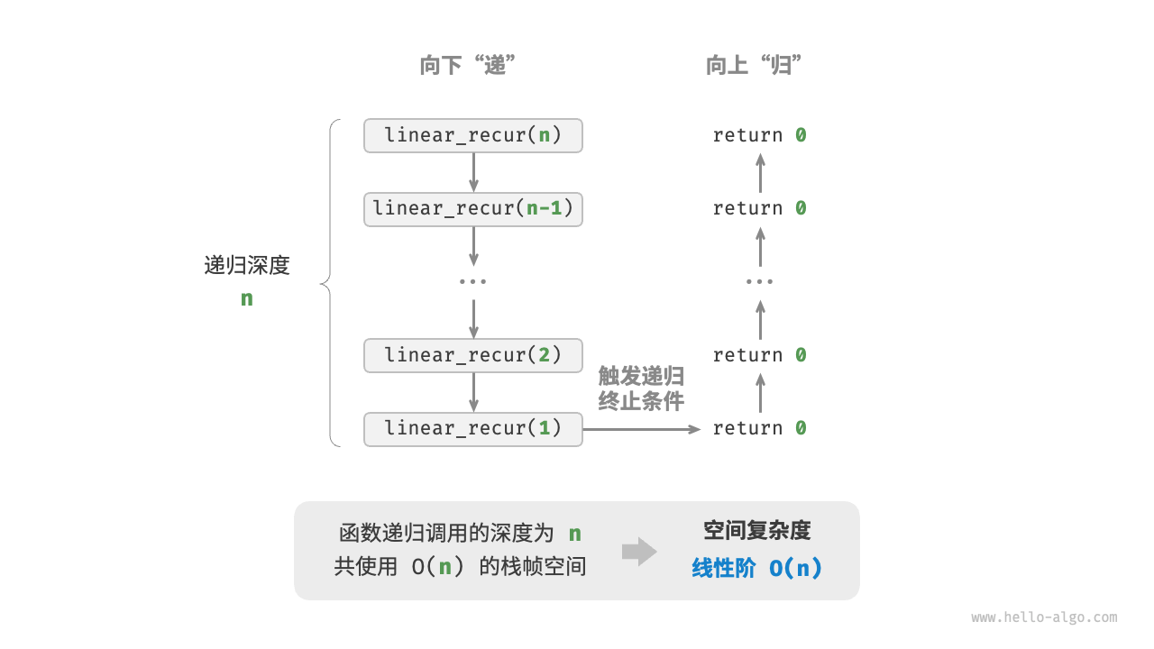
Figure 2-17 Linear order space complexity produced by recursive functions

3. Square order O(n2)

Square order is common in matrices and graphs, and the number of elements is related squarely to n:

/* 平方阶 */
void quadratic(int n) {
    // 二维列表占用 O(n^2) 空间
    int **numMatrix = malloc(sizeof(int *) * n);
    for (int i = 0; i < n; i++) {
        int *tmp = malloc(sizeof(int) * n);
        for (int j = 0; j < n; j++) {
            tmp[j] = 0;
        }
        numMatrix[i] = tmp;
    }

    // 内存释放
    for (int i = 0; i < n; i++) {
        free(numMatrix[i]);
    }
    free(numMatrix);
}

As shown in Figure 2-18, the recursion depth of this function is n. In each recursive function, an array is initialized with lengths of n, n−1,...,2,1, and the average length is n/2. Therefore, the total space occupied is O(n2):

/* 平方阶（递归实现） */
int quadraticRecur(int n) {
    if (n <= 0)
        return 0;
    int *nums = malloc(sizeof(int) * n);
    printf("递归 n = %d 中的 nums 长度 = %d\r\n", n, n);
    int res = quadraticRecur(n - 1);
    free(nums);
    return res;
}

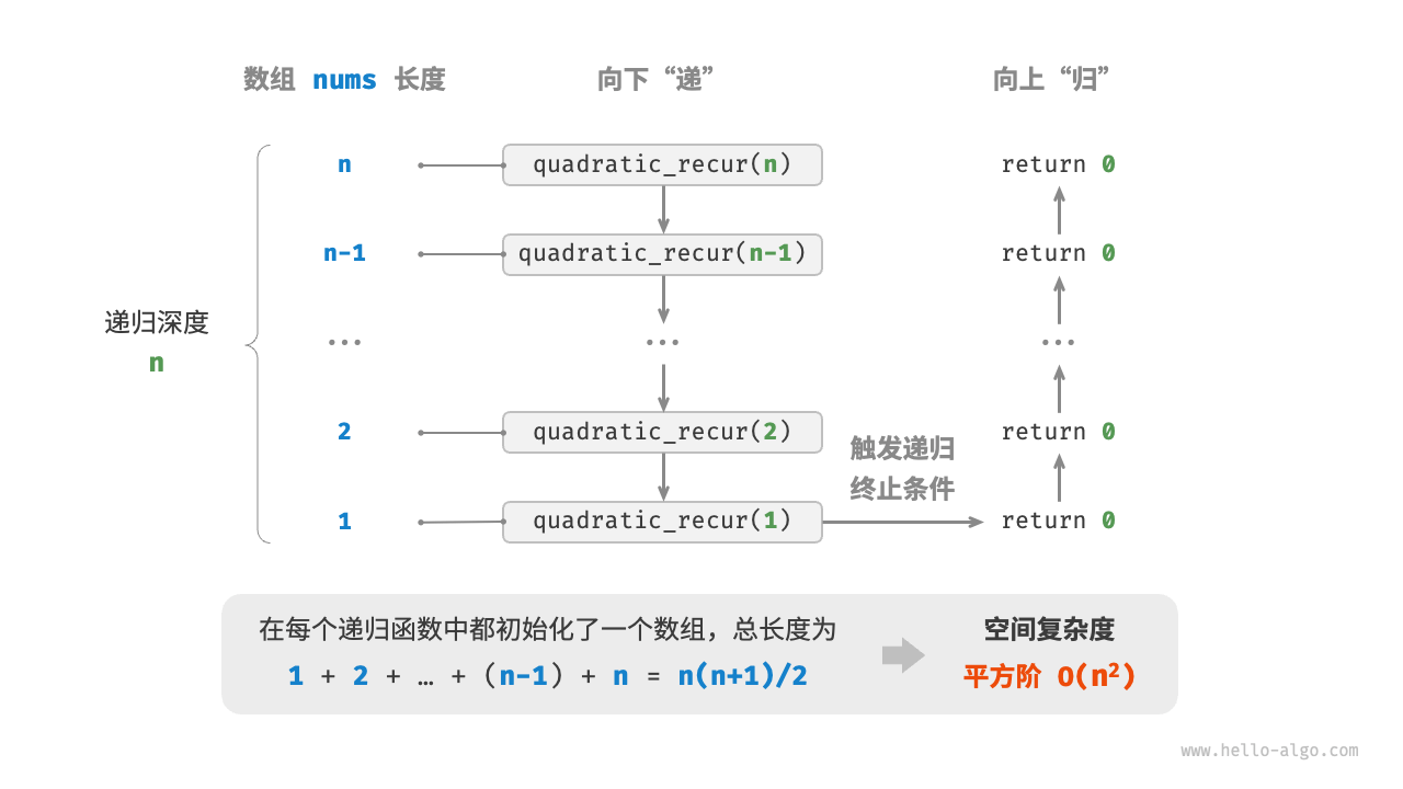
Figure 2-18 Square-order space complexity produced by recursive functions

4. Exponential order O(2n)

Exponential order is common in binary trees. Observing Figure 2-19, the number of nodes of a "full binary tree" with height n is 2n−1 and takes up O(2n) space:

/* 指数阶（建立满二叉树） */
TreeNode *buildTree(int n) {
    if (n == 0)
        return NULL;
    TreeNode *root = newTreeNode(0);
    root->left = buildTree(n - 1);
    root->right = buildTree(n - 1);
    return root;
}

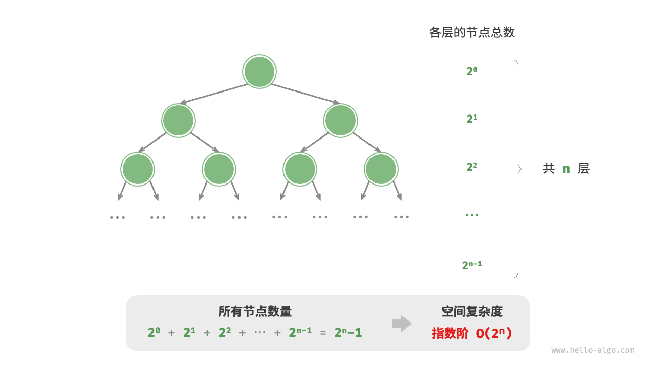
Figure 2-19 The exponential space complexity generated by a full binary tree

5. Logarithmic order O(log⁡n)

The logarithmic order is common in divide-and-conquer algorithms. For example, merge sorting inputs an array of length n. Each round of recursion divides the array into two halves at the midpoint, forming a recursive tree with a height of log⁡n, using O(log⁡n) stack frame space.

4.4 Trade-off between time and space

Ideally, we hope that the time complexity and space complexity of the algorithm can be optimized. However, in practical situations, it is often very difficult to optimize both time complexity and space complexity simultaneously.

Reducing time complexity usually comes at the expense of increasing space complexity, and vice versa . We call the idea of sacrificing memory space to improve the running speed of the algorithm "exchanging space for time"; conversely, it is called "exchanging time for space".

Which idea to choose depends on which aspect we value more. In most cases, time is more valuable than space, so "trade space for time" is usually the more common strategy. Of course, when the amount of data is large, it is also very important to control the space complexity.

5 Summary

1. Key review

Algorithm efficiency evaluation

Time efficiency and space efficiency are the two main evaluation indicators to measure the quality of the algorithm.
We can evaluate algorithm efficiency through actual testing, but it is difficult to eliminate the impact of the test environment and consumes a lot of computing resources.
Complexity analysis can overcome the shortcomings of actual testing. The analysis results are applicable to all running platforms and can reveal the efficiency of the algorithm under different data scales.

time complexity

Time complexity is used to measure the trend of algorithm running time increasing with the amount of data. It can effectively evaluate the efficiency of the algorithm, but it may fail in some cases. For example, when the amount of input data is small or the time complexity is the same, the algorithms cannot be accurately compared. The pros and cons of efficiency.
The worst time complexity is represented by big O notation, which corresponds to the asymptotic upper bound of the function, reflecting the growth level of the number of operations T(n) as n approaches positive infinity.
Estimating the time complexity is divided into two steps. First, count the number of operations, and then determine the asymptotic upper bound.
Common time complexities arranged from small to large are O(1), O(log⁡n), O(n), O(nlog⁡n), O(n2), O(2n) and O(n!), etc.
The time complexity of some algorithms is not fixed but depends on the distribution of the input data. Time complexity is divided into worst, best, and average time complexity. The best time complexity is rarely used because the input data generally needs to meet strict conditions to achieve the best situation.
The average time complexity reflects the operating efficiency of the algorithm under random data input and is closest to the algorithm performance in practical applications. Calculating the average time complexity requires statistical input data distribution and the mathematical expectation after synthesis.

space complexity

Space complexity functions similarly to time complexity and is used to measure the tendency of an algorithm to occupy space as the amount of data increases.
The relevant memory space during the operation of the algorithm can be divided into input space, temporary storage space and output space. Normally, the input space is not included in the space complexity calculation. The temporary storage space can be divided into instruction space, data space, and stack frame space. The stack frame space usually only affects the space complexity in recursive functions.
We usually only focus on the worst space complexity, that is, the space complexity of the statistical algorithm under the worst input data and worst running time point.
Common space complexities arranged from small to large include O(1), O(log⁡n), O(n), O(n2) and O(2n).

2. Q & A

Is the space complexity of tail recursion O(1)?

Theoretically, the space complexity of tail recursive functions can be optimized to O(1). However, most programming languages (such as Java, Python, C++, Go, C#, etc.) do not support automatic optimization of tail recursion, so the space complexity is usually considered to be O(n).

What is the difference between the terms function and method?

Functions can be executed independently, with all parameters passed explicitly. A method is associated with an object, is implicitly passed to the object that calls it, and can operate on the data contained in the instance of the class.

Below are some common programming languages.

C language is a procedural programming language and has no object-oriented concept, so it only has functions. But we can simulate object-oriented programming by creating a structure (struct), and the functions associated with the structure are equivalent to methods in other languages.
Java and C# are object-oriented programming languages, and code blocks (methods) are usually part of a class. A static method behaves like a function in that it is bound to the class and cannot access specific instance variables.
C++ and Python support both procedural programming (functions) and object-oriented programming (methods).

Does the figure "Common Space Complexity Types" reflect the absolute size of the occupied space?

No, the image shows space complexity, which reflects growth trends rather than the absolute size of the space occupied.

Assuming n=8, you may find that the value of each curve does not correspond to the function. This is because each curve contains a constant term that compresses the range of values into a visually comfortable range.

In practice, because we usually do not know the "constant term" complexity of each method, we generally cannot choose the optimal solution under n=8 based on complexity alone. But it is a good choice for n=85, when the growth trend is already dominant.