[PaddlePaddle] [Study Notes] PaddlePaddle official documentation - ① Use Python and NumPy to build a neural network model; ② Use PaddlePaddle to predict Boston housing prices

1. Overview of machine learning and deep learning

1.1 The relationship between artificial intelligence, machine learning, and deep learning

The concepts of artificial intelligence, machine learning and deep learning have been very popular in recent years, but many practitioners have difficulty explaining the relationship between them, and laymen are even more confused. Before studying deep learning, let’s start with the origins of the three concepts. In summary, the technical categories covered by artificial intelligence, machine learning and deep learning are gradually decreasing. The relationship between the three is as shown in the figure below, namely: artificial intelligence > machine learning > deep learning.

Artificial Intelligence (AI) is the broadest concept. It is a new technical science that develops theories, methods, technologies and application systems for simulating, extending and expanding human intelligence. Since this definition only states the goal and does not limit the method, there are many methods and branches to achieve artificial intelligence, causing it to become a "hodgepodge" discipline. Machine Learning (ML) is currently a relatively effective way to implement artificial intelligence. Deep Learning (DL) is the most popular branch of machine learning algorithms. It has made significant progress in recent years and has replaced most traditional machine learning algorithms.

1.2 Machine Learning

Different from artificial intelligence, machine learning, especially supervised learning, has a more clear reference. Machine learning is a specialized study of how computers can simulate or implement human learning behavior to acquire new knowledge or skills, reorganize existing knowledge structures, and continuously improve their performance. This sentence feels a bit "cloudy and foggy", which makes people confused. Let's analyze it from the two dimensions of machine learning implementation and methodology to help readers understand the ins and outs of machine learning more clearly.

1.2.1 Implementation of machine learning

The implementation of machine learning can be divided into two steps: ① training and ② prediction, similar to induction and deduction:

• Induction : Abstracting general rules from specific cases, the same is true for "training" in machine learning. From a certain number of samples (known model input $X$ and model output$Y$ ), learn to output$Y$ and input$The\; relationship\; between\; X$ (can be imagined as some kind of expression).

• Deduction : Deducing the results of specific cases from general rules, the same is true for "prediction" in machine learning. Based on YY obtained from training$Y$ andXXThe relationship between$X$$X$ , calculate the output$Y.$ _ Usually, if the output calculated by the model is consistent with the output of the real scene, the model is effective.

1.2.2 Machine learning methodology

The methodology of machine learning is similar to the process of human scientific research. The following takes "machine learning knowledge from Newton's second law experiment" as an example to help readers gain a deeper understanding of the essence of the methodology of machine learning (supervised learning), that is, in "machine learning" Three key elements of the model were identified during the “thinking” process:

1. hypothesis
2. evaluate
3. optimization

1.2.2.1 Case: Machine learns knowledge from Newton’s second law experiment

Newton's second law was proposed by Isaac Newton in his book "Mathematical Principles of Natural Philosophy" in 1687. Its common expression is: the acceleration of an object is directly proportional to the force, inversely proportional to the mass of the object, and inversely proportional to the mass of the object. Proportional to the reciprocal of mass . Newton's second law of motion and the first and third laws together form Newton's laws of motion, which describe the basic laws of motion in classical mechanics.

In middle school textbooks, there are two experimental design methods for Newton's second law: ① Inclined sliding method and ② Horizontal wire method, as shown in the figure.

相信很多读者都有摆弄滑轮和小木块做物理实验的青涩年代和美好回忆。通过多次实验数据，可以统计出如下表所示的不同作用力下的木块加速度。

次数	作用力 $X$	加速度 $Y$
1	4	2
2	4	2
…	…	…
n	6	3

观察实验数据不难猜测，物体的加速度 $a$ 和作用力 $F$ 之间的关系应该是线性关系。因此我们提出假设 $a=w\cdot F$，其中，$a$ 代表加速度，$F$ 代表作用力，$w$ 是待确定的参数。

通过大量实验数据的训练，确定参数 $w$ 是物体质量的倒数 $\frac{1}{m}$，即得到完整的模型公式 $a=F\cdot \frac{1}{m}$。当已知作用到某个物体的力时，基于模型可以快速预测物体的加速度。例如：燃料对火箭的推力 $F=10$，火箭的质量 $m=2$，可快速得出火箭的加速度 $a=5$。

1.2.2.2 如何确定模型参数？

这个有趣的案例演示了机器学习的基本过程，但其中有一个关键点的实现尚不清晰，即：如何确定模型参数 $w=\frac{1}{m}$？

确定参数的过程与科学家提出假说的方式类似，合理的假说可以最大化的解释所有的已知观测数据。如果未来观测到不符合理论假说的新数据，科学家会尝试提出新的假说。如：天文史上，使用大圆和小圆组合的方式计算天体运行，在中世纪是可以拟合观测数据的。但随着欧洲工业革命的推动，天文观测设备逐渐强大，已有的理论已经无法解释越来越多的观测数据，这促进了使用椭圆计算天体运行的理论假说出现。因此，模型有效的基本条件是能够拟合已知的样本，这给我们提供了学习有效模型的实现方案。

上图是以 $H$ 为模型的假设，它是一个关于参数 $w$ 和输入 $x$ 的函数，用 $H(w,x)$ 表示。模型的优化目标是 $H(w,The\; output\; of\; x)$ and the real output$Y$ should be as consistent as possible, and the difference between the two is the evaluation function of the model effect (the smaller the difference, the better).

Then, the process of determining parameters is to continuously reduce the evaluation function ( $H$和$Y$ gap) process. Until the model learns a parameter$w$ , which minimizes the value of the evaluation function.The evaluation function that measures the difference between the model's predicted value and the true value is also called the loss function (Loss).

Suppose the machine learns knowledge (model parameters ww ) by trying to answer (minimize loss) a large number of exercises (known samples) correctly$w$ ), and expect the model H ( w , x ) H(w,x)represented by the learned knowledge$H(w,x)$ , answer exam questions for which you don’t know the answer (unknown sample). Minimizing loss is the optimization goal of the model.The method to achieve loss minimization is called an optimization algorithm, also known as a solution-finding algorithm (finding the parameter solution that minimizes the loss function). Parameter$w$ and enter$The\; basic\; structure\; that\; makes\; up\; a\; formula$ is called a hypothesis. In the case of Newton's second law, based on the observation of the data, we proposed a linear hypothesis, that is, the force and acceleration are linearly related, expressed by a linear equation. It can be seen that ①model assumptions, ②evaluation function(loss/optimization objective) and ③optimization algorithmare the three key elements that constitute the model.

1.2.2.3 Model structure

How do model assumptions, evaluation functions and optimization algorithms support the machine learning process? As shown below.

• Model hypothesis : There are thousands of possible relationships in the world, aimless exploration $Y\leftarrow The\; relationship\; between\; X$ is obviously very inefficient. Therefore, the hypothesis space first delimits the possible relationships that a model can express, as shown in the blue circle. The machine will further search for the optimal Y ← XY \leftarrow Xwithin the hypothetically circled circle$Y\leftarrow X$ relationship, that is, determining the parameter$w$。
• Evaluation function : Before looking for the optimal, we need to define what is optimal, that is, evaluate a $Y\leftarrow$An indicator of the quality of the$X\; relationship.$It is usually measured whether the relationship can fit the existing observation samples well, and the minimum fitting error is taken as the optimization goal.
• Optimization algorithm : After setting the evaluation index, within the range circled by the hypothesis, $Y\leftarrow$Find the$X\; relationship,\; and\; this\; method\; of\; finding\; the\; optimal\; solution\; is\; the\; optimization\; algorithm.$The stupidest optimization algorithm is to calculate the loss function by exhaustively enumerating every possible value according to the possible parameters, and retain the parameters that minimize the loss function as the final result.

From the above process, it can be concluded that the machine learning process is basically consistent with the learning process of Newton's second law, and is divided into three stages: hypothesis , evaluation and optimization :

• Hypothesis : By observing the acceleration $a$ and forceFFObservation data of$F$$a$ and$F$ is a linear relationship, that is,$a=w\cdot F$。
• Evaluation : The fitting effect on known observation data is good, that is, $w\cdot The\; result\; of\; F$ calculation should be consistent with the observed$a$ as close as possible.
• Optimization : in parameter wwAmong all possible values ​​of$w$$w=\frac{1}{m}$It can make the evaluation the best (best fit the observed sample).

The framework for machines to perform learning tasks reflects that the essence of learning is "parameter estimation" (Learning is parameter estimation)。

The above methodology uses a more standardized representation as shown in the figure below, the unknown objective function $f$ , with training samples$D=(x_1,y_1),(x_2,y_2),...,(x_n,y_n)$ is based on. From the hypothesis set$In\; H$ , through learning algorithm$A$ finds a function$g$ . if$g$ can best fit the training sample$D$ , then the function$g$ is close to the objective function$f$。

On this basis, many seemingly completely different problems can be learned using the same framework, such as scientific laws, image recognition, machine translation and automatic question answering, etc.Their learning goals are to fit a "big formula $f$”,As shown below.

1.3 Deep learning

The theory of machine learning algorithms matured in the 1990s and achieved success in many fields, but the quiet days only lasted until about 2010. With the emergence of big data and the improvement of computer computing power, deep learning models have emerged, which has greatly changed the application landscape of machine learning. Today, most machine learning tasks can be solved using deep learning models. Especially in fields such as speech, computer vision, and natural language processing, the effects of deep learning models are significantly improved compared to traditional machine learning algorithms .

Compared with traditional machine learning algorithms, what improvements has deep learning made? In fact, the two are consistent in theoretical structure, namely: model assumptions, evaluation functions and optimization algorithms . The fundamental difference lies in the complexity of the assumptions . As shown in the second example (image recognition) in the figure above, for photos of beautiful women, the human brain can receive colorful optical signals and can quickly respond that the picture is of a beautiful woman. But for a computer, it can only receive a digital matrix. For a high-level semantic concept like beauty, the complexity of information transformation from pixels to high-level semantic concepts is unimaginable. This conversion process is shown in the figure below . Show.

This transformation can no longer be expressed using mathematical formulas, so researchers drew on the structure of human brain neurons and designed a neural network model, as shown in the figure below.

Figure (a) shows the design of the basic unit of the neural network - the perceptron. The way it processes information is very similar to a single neuron in the human brain; Figure (b) shows several classic The neural network structure (will be explained in detail in subsequent chapters) is similar to the various organs with different functions formed based on a large number of neuron connections in the human brain.

1.3.1 Basic concepts of neural networks

Artificial neural networks include multiple neural network layers, such as: Convolution Layer, Fully Connected Layer, LSTM (Long Short-Term Memory, Long Short-Term Memory Network), etc. Each layer includes many Neurons, nonlinear neural networks with more than three layers can be called deep neural networks (D-CNN). In layman's terms, a deep learning model can be regarded as a mapping function from input to output, such as the mapping of images to high-level semantics (beauty). A deep enough neural network can theoretically fit any complex function . Therefore, neural networks are very suitable for learning the inherent laws and representation levels of sample data, and have good applicability to text, image and speech tasks. The tasks in these fields are the basic modules of artificial intelligence, so it is not surprising that deep learning is called the basis for realizing artificial intelligence. The basic structure of the neural network (NN) is shown in the figure below.

in:

• Neuron : Each node in the neural network is called a neuron and consists of two parts:
  1. Weighted sum : weighted sum of all inputs.
  2. Nonlinear transformation (activation function) : The result of the weighted sum is transformed by a nonlinear function, allowing neuron calculations to have nonlinear capabilities.
• Multi-layer connection : A large number of such nodes are arranged at different levels and connected to form a multi-layer structure, which is called a neural network.
• Forward calculation : The process of calculating output from input, in order from front to back of the network.
• Computational graph : Graphically displaying the computational logic of a neural network is also called a computational graph. The computational graph of a neural network can also be expressed in the form of a formula: Y = f 3 ( f 2 ( f 1 ( w 1 ⋅ x $$Y=f_3(f_2(f_1(w_1\cdot x_1+w_2\cdot x_2+w_3\cdot x_3+b)+...)+...)$$

It can be seen that the neural network (NN) is not that mysterious. Its essence is a "big formula" containing many parameters .

1.3.2 The development history of deep learning

The idea of ​​neural networks was proposed more than 70 years ago, and today's design theories of neural networks and deep learning are becoming more and more perfect step by step. In these long years of development, some shining moments of key breakthroughs are worth remembering by deep learning enthusiasts, as shown in the figure below.

• 1940s : The structure of a neuron is first proposed, but the weights are not learnable.
• 1950s-1960s : The weight learning theory was proposed, and the neuron (Neuron) structure tended to be perfect, opening the first golden age of neural networks (NN).
• 1969 : The XOR problem was raised (people were surprised to find that the neural network model could not solve even simple XOR problems, and their expectations fell from the clouds to the bottom), and the neural network model entered the dark age of being shelved.
• 1986 : The newly proposed multi-layer neural network solved the XOR problem. However, with the rise of machine learning models such as SVM with more complete theories and better practical results after the 1990s, neural networks did not receive attention.
• Around 2010 : Deep learning enters its real rise. As the technology of improved neural network models shines in speech and computer vision tasks, it has gradually been proven to be more effective in more tasks, such as natural language processing (NLP) and massive data tasks. At this point, the neural network model has been reborn and has a more famous name: Deep Learning.

Why didn’t neural networks come to life until 2010? This is related to the prerequisites on which the success of deep learning depends: ① emergence of big data, ② hardware development and ③ algorithm optimization.

1. The emergence of big data : Big data is an effective prerequisite for the development of neural networks. Neural networks (NN) and deep learning (DL) are very powerful models that require sufficient amounts of training data. Today, the reason why many traditional machine learning algorithms and artificial features are still effective enough is that in many scenarios there is not enough labeled data to support deep learning. The ability of deep learning is particularly like the heroic words of the scientist Archimedes: "Give me a lever long enough, and I can move the earth!". Deep learning can also make similar claims: "Give me enough data and I can learn any complex relationship." But in reality, long enough leverage, like enough data, can often be nothing more than a rosy vision. It was not until recent years that the IT level of various industries has increased and the amount of accumulated data has increased explosively, making it possible to apply deep learning models.
2. Hardware development and algorithm optimization : Rely on hardware development and algorithm optimization. At this stage, relying on more powerful computers, GPUs, autoencoder pre-training and parallel computing technologies, the difficulties of deep learning in model training have been gradually overcome. Among them, data volume and hardware are the more important reasons. Without the first two, scientists would be unable to optimize the algorithm.

1.3.3 Research and application of deep learning are booming

As early as 1998, some scientists had used neural network models to recognize handwritten digit images (MNIST). However, the rise of deep learning in computer vision applications began with the use of AlexNet for image classification in the 2012 ImageNet competition. If you compare the 1998 and 2012 models, you will find that the two are very similar in network structure, with only some optimizations in details. In the past 14 years, the substantial improvement in computing performance and the explosive growth in data volume have prompted the model to complete the leap from "simple number recognition" to "complex image classification".

Although it has a long history, deep learning is still booming today. On the one hand, basic research is developing rapidly, and on the other hand, industrial practices are emerging in endlessly. Based on statistics from ICLR (International Conference on Learning Representations), the top conference on deep learning, the number of papers related to deep learning is increasing year by year, as shown in the figure below. At the same time, not only deep learning conferences, but also a large number of papers from international conferences such as ICML and KDD related to data and model technology, CVPR focusing on vision, and EMNLP focusing on natural language processing, all involve deep learning technology. Research in this field and related fields is in the ascendant, and technology is still undergoing innovation and breakthroughs.

On the other hand, artificial intelligence technology based on deep learning has extremely broad application scenarios in upgrading and transforming many traditional industry fields. The picture below is taken from a research report by iResearch. Artificial intelligence technology can not only be applied in many industries (breadth), but also has achieved market realization in some industries (such as security, remote sensing, Internet, finance, industry, etc.) and rapid growth (depth), contributing huge economic value to society.

As shown in the figure below, taking the industry application distribution of computer vision (CV) as an example, according to IDC statistics and forecasts, with the penetration of artificial intelligence into various industries, the proportion of the output value of the Internet industry that currently uses artificial intelligence has increased. will gradually become smaller.

1.3.4 Deep learning has changed the research and development model of AI applications

1.3.4.1 Implemented end-to-end (End2End) learning

Deep learning has changed the implementation model of algorithms in many fields. Before the rise of deep learning, the idea of ​​modeling in many fields was to invest a lot of energy in feature engineering, precipitate experts' "artificial understanding" of a certain field into feature expressions, and then use simple models to complete tasks (such as classification or regression). When there is sufficient data, the deep learning model can achieve end-to-end (End2End) learning, that is, no special feature engineering is required . The original features are input into the model, and the model can complete feature extraction and classification tasks at the same time, as shown below. shown.

Taking computer vision tasks as an example, feature engineering is a series of computational steps for extracting features designed by many image scientists based on human understanding of visual theory, typically such as SIFT features. In the field of computer vision before 2010, people generally used SIFT-type features + SVM-type simple shallow models to complete modeling tasks.

Description :

1. SIFT features were proposed by David Lowe in 1999 and refined in 2004. SIFT features are based on some local appearance interest points on the object and are independent of the size and rotation of the image. The tolerance for light, noise, and micro-viewing angle changes is also quite high. Based on these characteristics, they are highly salient and relatively easy to retrieve. In a large feature database, objects are easily identified and misidentification is rare. The detection rate for partial object occlusion using SIFT feature description is also quite high, and even more than 3 SIFT object features are enough to calculate the position and orientation. Under the conditions of today's computer hardware speed and small feature database, the recognition speed can be close to real-time operation. SIFT features have a large amount of information and are suitable for fast and accurate matching in massive databases.

2. The most essential difference between deep learning and traditional machine learning is the need for feature engineering：

   • In traditional machine learning, feature engineering is an important step that requires domain experts to manually design and select relevant features from raw data as input for use by machine learning algorithms. This process often requires significant domain knowledge, data preprocessing, and manual effort to create informative, meaningful data representations.
   • Deep learning can automatically learn relevant features from original data during the training process. Deep learning models, especially neural networks, are able to gradually learn hierarchical representations of data through multiple levels of computation. This ability to automatically learn features makes deep learning more suitable for processing complex and high-dimensional data.

1.3.4.2 Achieved standardization of deep learning framework

In addition to its wide range of applications, deep learning also promotes artificial intelligence into the stage of industrial mass production. The versatility of the algorithm leads to the creation of standardized, automated and modular frameworks, as shown in the figure below.

Prior to this, different schools of machine learning algorithms had different theories and implementations, resulting in each algorithm having to be implemented independently, such as Random Forest (RF) and Support Vector Machine (SVM). However, under the deep learning framework, the algorithm structures of different models have great versatility, such as the convolutional neural network model (CNN) commonly used in computer vision and the long short-term memory model (LSTM) commonly used in natural language processing. It is divided into networking module, gradient descent optimization module and prediction module. This makes it possible to abstract a unified framework and greatly reduces the cost of writing modeling code. Some relatively common modules, such as the implementation of basic network operators and various optimization algorithms, can be implemented by the framework. Modelers only need to focus on data processing, configuring networking, and tying together the training and prediction processes with a small amount of code.

Before the emergence of deep learning frameworks, machine learning engineers were in the era of "manual workshop" production. In order to complete the modeling, engineers need to reserve a lot of mathematical knowledge and accumulate a lot of industry knowledge for feature engineering work. Each model is extremely personalized, and the modeler, like a craftsman, forms his or her own accumulation into a "personalized signature" of the model. Nowadays, "deep learning engineers" have entered the era of industrialized mass production. As long as they master the necessary but small theoretical knowledge of deep learning and master Python programming, they can implement very effective models on the deep learning framework, even with the most leading models in the field. On par. Technical barriers in the field of modeling are facing subversion, which is also an opportunity for new entrants.

1.4 There is broad space for career development in artificial intelligence

下面就从经济回报的视角，分析下人工智能是不是一个有前途的职业。坦率的说，如巴菲特所言，选择一个自己喜欢的职业是真正的好职业。但对于多数普通人，经济回报也是职业选择的重要考虑因素。一个有高经济回报的职业一定是市场需求远远大于市场供给的职业，且市场需求要保持长期的增长，而市场供给难以中短期得到补充。

1.4.1 人工智能岗位的市场需求旺盛

根据各大咨询公司的行业研究报告，人工智能相关产业在未来十年预计有 30% ~ 40% 的年增长率。一方面，人工智能的应用会从互联网行业逐渐扩展到金融、工业、农业、能源、城市、交通、医疗、教育等更广泛的行业，应用空间和潜力巨大；另一方面，受限于工智能技术本身的成熟度以及人工智能落地要结合场景的数据处理、系统改造和业务流程优化等条件的制约，人工智能应用的价值释放过程会相对缓慢。这使得市场对人工智能的岗位需求形成了一条稳步又长期增长的曲线，与互联网行业相比，对多数的求职者更加友好，如下图所示。

互联网行业由于技术成熟周期短，应用落地的推进速度快，反而形成一条增长率更高（年增长率超过 100%）但增长周期更短的曲线（电脑互联网时代 10 年，移动互联网时代 10 年）。当行业增长达到顶峰，对岗位的需求也会相应回落，如同 2021 年底的互联网行业的现状。

1.4.2 复合型人才成为市场刚需

在人工智能落地到千行万业的过程中，企业需求量最大、也最为迫切的是既懂行业知识和场景，又懂人工智能理论，还具备实践能力和经验的“复合型人才”。成为“复合型人才”不仅需要学习书本知识，还要大量进行产业实践，使得这种人才有成长深度，供给增长缓慢。从上述分析可见，当人工智能产业在未来几十年保持稳定的增长，而产业需要的“复合型人才”又难以大量供给的情况下，人工智能应用研发岗位会维持一个很好的经济回报。

2. 使用 Python 和 NumPy 构建神经网络模型

In the last chapter, we had a preliminary understanding of the basic concepts of neural networks (such as neurons, multi-layer connections, forward calculations, calculation graphs) and the three elements of the model structure (model assumptions, evaluation functions and optimization algorithms). This chapter will take the "Boston housing price prediction" task as an example to introduce the thinking process and operation method of using Python and NumPy to build a neural network model.

Boston house price prediction is a classic machine learning task, similar to the "Hello World" of the programmer's world. As everyone generally knows about housing prices, housing prices in the Boston area are affected by many factors. This data set counts 13 factors that may affect housing prices and the average price of houses of this type. It is expected to build a model for predicting housing prices based on 13 factors, as shown in the figure below.

For prediction problems, it can be divided into ① regression tasks and ② classification tasks according to whether the type of prediction output is continuous real values ​​or discrete labels. Because house prices are a continuous value, house price prediction is obviously a regression task. Below we try to solve this problem with the simplest linear regression model and use a neural network to implement this model.

2.1 Linear Regression model

Assume that the relationship between housing prices and various influencing factors can be described by a linear relationship:

$$y=\sum _{j=1}^M{x}_j{w}_j+b\text{\hspace{1em}(1)}$$

The solution of the model is to fit each $w_j$andbb $b$ . Among them,$w_j$andbb $b$ respectively represent the weight (Weight) and bias (Bias) of the linear model. In the one-dimensional case,$w_j$andbb $b$ is the slope and intercept of the line.

The linear regression model uses the mean squared error (MSE) as the loss function (Loss) to measure the difference between the predicted house price and the real house price. The formula is as follows:

$$\mathrm{MSE}=\frac{1}{n}\sum _{i=1}^n({\hat{Y}}_i-Y_i{)}^2\text{\hspace{1em}(2)}$$

Think :

Why use mean square error (MSE) as the loss function? The accuracy of the overall sample is measured by summing the prediction errors of the model on each training sample. This is because the design of the loss function not only needs to consider "rationality", but also needs to consider "ease of solution". This issue will be elaborated on in the following content.

---

In the standard structure of the neural network, each neuron (Neuron) is composed of a weighted sum and a nonlinear transformation, and then multiple neurons are placed and connected in layers to form a neural network (NN). The linear regression model can be considered a minimalist special case of the neural network model. It is a neuron with only a weighted sum and no nonlinear transformation (no need to form a network), as shown in the figure below.

2.2 Use Python and NumPy to implement the Boston housing price prediction task

Deep learning not only realizes end-to-end learning of models, but also promotes artificial intelligence into the stage of industrial mass production, producing a universal framework for standardization, automation, and modularization. Deep learning models in different scenarios have a certain degree of versatility, and the construction and training of the model can be completed in five steps, as shown in the figure below.

It is precisely because of the universality of the modeling and training process of deep learning that when building different models, only the three elements of the model are different and the other steps are basically the same, so the deep learning framework can be useful.

2.2.1 Data processing

数据处理包含五个部分：①数据导入、②数据形状变换、③数据集划分、④数据归一化处理和⑤封装 load_data 函数。数据一般只有经过预处理后，才能被模型调用。

2.2.1.1 读入数据

通过如下代码读入数据，了解下波士顿房价的数据集结构，数据存放在本地目录下 housing.data 文件中。

数据集下载地址：http://paddlemodels.bj.bcebos.com/uci_housing/housing.data

import numpy as np
import json


# 读取数据
datafile = "/data/data_01/lijiandong/Datasets/boston_house_price/housing.data"
data = np.fromfile(datafile, sep=" ")
print(data)  # /data/data_01/lijiandong/Datasets/boston_house_price/housing.data
print(data.shape)  # (7084,)

2.2.1.2 数据形状变换

由于读入的原始数据是 1 维的，所有数据都连在一起。因此需要我们将数据的形状进行变换，形成一个 2 维的矩阵，每行为一个数据样本（有 14 个列），每个数据样本包含 13 个 $X$（影响房价的特征）和一个 $Y$（该类型房屋的均价）。

"""
读入之后的数据被转化成1维array，其中array的第0-13项是第一条数据，第14-27项是第二条数据，以此类推.... 
这里对原始数据做reshape，变成N x 14的形式
"""
feature_names = [ 'CRIM', 'ZN', 'INDUS', 'CHAS', 'NOX', 'RM', 'AGE','DIS', 'RAD', 'TAX', 'PTRATIO', 'B', 'LSTAT', 'MEDV' ]
feature_num = len(feature_names)
data = data.reshape([data.shape[0] // feature_num, feature_num])

# 查看数据
x = data[0]  # 取第一行
print(x.shape)  # (14,)
print(x)
"""
[6.320e-03 1.800e+01 2.310e+00 0.000e+00 5.380e-01 6.575e+00 6.520e+01
 4.090e+00 1.000e+00 2.960e+02 1.530e+01 3.969e+02 4.980e+00 2.400e+01]
"""

2.2.1.3 数据集划分

将数据集划分成训练集和测试集，其中训练集用于确定模型的参数，测试集用于评判模型的效果。为什么要对数据集进行拆分，而不能直接应用于模型训练呢？这与学生时代的授课和考试关系比较类似，如下图所示。

上学时总有一些自作聪明的同学，平时不认真学习，考试前临阵抱佛脚，将习题死记硬背下来，但是成绩往往并不好。因为学校期望学生掌握的是知识，而不仅仅是习题本身。另出新的考题，才能鼓励学生努力去掌握习题背后的原理。同样我们期望模型学习的是任务的本质规律，而不是训练数据本身，模型训练未使用的数据，才能更真实的评估模型的效果。

在本案例中，我们将 80% 的数据用作训练集，20% 用作测试集，实现代码如下。

ratio = 0.8
offset = int(data.shape[0] * ratio)
training_data = data[:offset]
test_data = data[offset:]

print(data.shape)  # (506, 14)
print(training_data.shape)  # (404, 14)
print(test_data.shape)  # (102, 14)

通过打印训练集的形状，可以发现共有 404 个样本，每个样本含有 13 个特征和 1 个预测值。

2.2.1.4 数据归一化处理

Data normalization is a common data preprocessing technique used to scale data to a certain range, usually $[0,1]$ or$[-1,1]$ (the former is more widely used, so we use the former). The formula for data normalization is as follows:

For each feature (or each column), assume that the range of the original data is $[\min ,\max ]$ , the normalized data can be calculated by the following formula:

$$Normalized\; value=\frac{original\; value-\min }{\max -\min }$$

Among them, "original value" refers to the original data value in a specific feature, "min" is the minimum value of the feature in the data set, and "max" is the maximum value of the feature in the data set.

Use normalization to scale the value of each feature to $[0,1]$ between. This has two benefits:

1. Model training is more efficient, which will be explained in detail in the second half of this section;
2. The weight before a feature can represent the contribution of the variable to the prediction result (because each feature value itself has the same range).

# 计算train数据集的最大值和最小值
maxinums, minimus = training_data.max(axis=0), training_data.min(axis=0)

# 对数据进行归一化处理
for col_name in range(feature_num):
    # 训练集归一化
    training_data[:, col_name] = (training_data[:, col_name] - minimus[col_name]) / (maxinums[col_name] - minimus[col_name])
    # 测试集归一化（确保了测试集上的数据也使用了与训练集相同的归一化转换，避免了引入测试集信息污染）
    test_data[:, col_name] = (test_data[:, col_name] - minimus[col_name]) / (maxinums[col_name] - minimus[col_name])

# 验证是否有大于1的值
print(np.any(training_data[:, :-1] > 1.0))  # False
print(np.any(test_data[:, :-1] > 1.0))  # True（这是正常的，因为我们使用了训练集的归一化参数）

2.2.1.5 Encapsulate into load_datafunctions

Encapsulate the above data processing operations into load_datafunctions for the next step of calling the model. The implementation method is as follows.

import numpy as np
import json


def data_load():
    # 2.2.1.1 读入数据
    datafile = "/data/data_01/lijiandong/Datasets/boston_house_price/housing.data"
    data = np.fromfile(datafile, sep=" ")


    # 2.2.1.2 数据形状变换
    feature_names = [ 'CRIM', 'ZN', 'INDUS', 'CHAS', 'NOX', 'RM', 'AGE','DIS', 'RAD', 'TAX', 'PTRATIO', 'B', 'LSTAT', 'MEDV' ]
    feature_num = len(feature_names)
    data = data.reshape([data.shape[0] // feature_num, feature_num])  # [N, 14]


    # 2.2.1.3 数据集划分
    ratio = 0.8
    offset = int(data.shape[0] * ratio)
    training_data = data[:offset]
    test_data = data[offset:]


    # 2.2.1.4 数据归一化处理
    # 计算train数据集的最大值和最小值
    maxinums, minimus = training_data.max(axis=0), training_data.min(axis=0)

    # 对数据进行归一化处理
    for col_name in range(feature_num):
        # 训练集归一化
        training_data[:, col_name] = (training_data[:, col_name] - minimus[col_name]) / (maxinums[col_name] - minimus[col_name])
        # 测试集归一化（确保了测试集上的数据也使用了与训练集相同的归一化转换，避免了引入测试集信息污染）
        test_data[:, col_name] = (test_data[:, col_name] - minimus[col_name]) / (maxinums[col_name] - minimus[col_name])
        
    return training_data, test_data


# 获取数据
training_data, test_data = data_load()
x = training_data[:, :-1]  # 训练数据
target = training_data[:, -1:]  # 目标值

# 查看数据
print(f"x.shape: {
      
      x.shape}")  # (404, 13)
print(f"target.shape: {
      
      target.shape}")  # (404,)

2.2.2 Model design

Model design is one of the key elements of a deep learning model. It is also called network structure design. It is equivalent to the hypothesis space of the model, that is, the process of realizing the "forward calculation" (from input to output) of the model.

If both the input feature and the output predicted value are expressed as vectors, the input feature $x$ has 13 components,$y$ has 1 component, then the shape of the parameter weight is$13\times 1$ . Suppose we initialize the parameters with any number as follows:

$$w=[0.1,0.2,0.3,0.4,0.5,0.6,0.7,0.8,-0.1,-0.2,-0.3,-0.4,0.0]$$

Expressed in code:

w = [0.1, 0.2, 0.3, 0.4, 0.5, 0.6, 0.7, 0.8, -0.1, -0.2, -0.3, -0.4, 0.0]
w = np.array(w).reshape([13, 1])

Take out the first sample data and observe the result of multiplying the sample's feature vector and parameter vector.

x1 = x[0]
t = np.dot(x1, w)
print(t)  # [0.69474855]

The complete linear regression formula also needs to initialize the offset $b$ , also assign an initial value of -0.2 arbitrarily. Then, the complete output of the linear regression model is$z=t+b$ . This process of calculating output values ​​from features and parameters is called "forward calculation".

b = -0.2  # bias
z = t + b
print(z)  # [0.49474855]

The above process of calculating prediction output is described in the form of "class and object". The class member variable has the parameter $w$ and$b$ . Complete the above calculation process from features and parameters to output predicted values ​​by writing aforwardfunction (representing "forward calculation"). The code is as follows.

class Network:
    def __init__(self, num_of_weights):
        np.random.seed(0)
        self.w = np.random.randn(num_of_weights, 1)  # 随机产生w的初始值
        self.b = 0.0  # 不使用偏置
        
    def forward(self, x):
        z = np.dot(x, self.w) + self.b
        return z

Based on the definition of the Network class, the calculation process of the model is as follows.

net = Network(13)
x1 = x[0]
y1 = target[0]
z = net.forward(x1)
print(z)  # [2.39362982]

From the above forward calculation process, we can see that linear regression can also be expressed as a simple neural network (only one neuron, and the activation function is the identity $y=y$ ). This is also the reason why machine learning models are generally replaced by deep learning models:due to the powerful representation capabilities of deep learning networks, the learning capabilities of many traditional machine learning models are equivalent to those of relatively simple deep learning models.

2.2.3 Training configuration

After the model design is completed, it is necessary to find the optimal value of the model through training configuration, that is, to measure the quality of the model through the loss function. Training configuration is also one of the key elements of deep learning models.

Calculate $x_1$The housing price corresponding to the influencing factors represented should be $z$ , but the actual data tells us that the house price is$y$ . At this time we need some kind of indicator to measure the predicted value$z$ and the true valueyythe difference between$y\; .$For regression problems, the most commonly used measurement method is to use the mean square error (MSE) as an indicator to evaluate the quality of the model. The specific definition is as follows:

$$\mathrm{Loss}=(y-z{)}^2\text{\hspace{1em}(3)}$$

Loss in the above formula (abbreviated as: $L$ ) is also often called the loss function, which is a measure of the quality of the model. Here we need to think about a question: If we want to measure the gap between predicted house prices and real house prices, can we just add the absolute value of the gap for each sample? The sum of the absolute values ​​of the differences is a more intuitive and simple idea. Why the sum of the squares?

This is because the design of the loss function must not only consider the "reasonableness" of accurately measuring the problem, but also usually consider the "ease of optimization and solution". As for the answer to this question, it will be revealed after the optimization algorithm is introduced.

In regression problems, mean square error (MSE) is a relatively common form. In classification problems, cross entropy (Cross Entropy) is usually used as the loss function, which will be introduced in more detail in subsequent chapters. The implementation of calculating the loss function value for a sample is as follows.

loss = (y1 - z) ** 2
print(loss)  # [3.88644793]

Because the loss function value of each sample needs to be taken into account when calculating the loss function, we need to sum the loss function of a single sample and divide it by the total number of samples $N$。

$$L=\frac{1}{N}\sum _{i=1}^N(y_i-z_i{)}^2\text{\hspace{1em}(4)}$$

The calculation process of adding the loss function under the Network class is as follows.

class Network:
    def __init__(self, num_of_weights):
        np.random.seed(0)
        self.w = np.random.randn(num_of_weights, 1)  # 随机产生w的初始值
        self.b = 0.0  # 不使用偏置
        
    def forward(self, x):
        z = np.dot(x, self.w) + self.b
        return z
    
    def loss(self, pred, gt):
        loss_value_sum = (pred - gt) ** 2
        return np.mean(loss_value_sum)

Using the defined Network class, the predicted value and loss function can be easily calculated. It should be noted that the variables in the class x, w, b, pred, gt, loss_value_sumare all vectors. Taking the variable xas an example, there are two dimensions, one represents the number of features (the value is 13), and the other represents the number of samples. The code is as follows.

# 组成向量一次性计算多个值
x1 = x[:3]  # 前三行
y1 = target[:3]  # 前三行

pred = net.forward(x1)
print(f"pred: {
      
      pred}")

loss = net.loss(pred, target)
print(f"loss: {
      
      loss}")

result:

pred: [[2.39362982]
 [2.46752393]
 [2.02483479]]
loss: 3.573658599044957

2.2.4 Training process

The above calculation process describes how to construct a neural network and complete the calculation of predicted values ​​and loss functions through the neural network. Next, we will introduce how to solve the parameter $w$ and$The\; value\; of\; b$ ,this process is also called the model training process. The training process is one of the key elements of the deep learning model, and its goal is to make the defined loss function$Loss$ should be as small as possible, that is to say find a parameter solution$w$ and$b$ , making the loss function obtain a minimum value.

Let’s do a small test first: As shown in the figure below, based on calculus knowledge, find that the slope of a curve at a certain point is equal to the derivative value of the function at that point. So think about it, when it is at the extreme point of the curve, what is the slope of that point?

This question is not difficult to answer. The slope at the extreme point of the curve is 0, that is, the derivative of the function at the extreme point is 0. Then, let the loss function take the minimum value of $w$ and$b$ should be the solution to the following system of equations:

$$\frac{\partial L}{\partial w}=0\text{\hspace{1em}(5)}$$

$$\frac{\partial L}{\partial b}=0\text{\hspace{1em}(6)}$$

where $L$ represents the value of the loss function,$w$ is the model weight,$b$ is the bias term. $w$ and$b$ are all model parameters to be learned.

Express the loss function in the form of a matrix, as follows:

$$L=\frac{1}{N}||y-(Xw+b)|{|}^2\text{\hspace{1em}(7)}$$

Among them $y$ is$A\; vector\; composed\; of\; label\; values\; of\; N$ samples, with a shape of$N\times 1$；$X$ isNNA matrix composed of$N$$N\times D$，$D$ is the data feature length;$w$ is a weight vector with a shape of$D\times 1$；$b$ means that all elements are$vector\; of\; b$ with shape$N\times 1$。

Calculation formula 7 for parameter bbPartial derivative of$b\; :$

$$\frac{\partial L}{\partial b}=1^T[y-(Xw+b)]\text{\hspace{1em}(8)}$$

Note that the above formula ignores the coefficient $\frac{2}{N}$, does not affect the final result. of which $1$ is$An\; N$ -dimensional all-1 vector.

Let formula 8 equal 0, we get

$$b^{\ast }={\overline{x}}^{T}w-\overline{y}\text{\hspace{1em}(9)}$$

其中$\overline{y}=\frac{1}{N}{1}^{T}y$is the average of all labels,$\overline{x}=\frac{1}{N}(1^{T}X{)}^T$ is the average of all feature vectors. Will$b^{\ast }$ is brought into formula 7 and the parameterwwTaking the partial derivative of$w\; ,\; we\; get$

$$\frac{\partial L}{\partial w}=(X-{\overline{x}}^T{)}^T[(y-\overline{y})-(X-{\overline{x}}^T)w]\text{\hspace{1em}(10)}$$

Let formula 10 equal 0 to get the optimal parameters

$$w^{\ast }=[(X-{\overline{x}}^T{)}^T(X-{\overline{x}}^T){]}^{-1}(X-{\overline{x}}^T{)}^T(y-\overline{y})\text{\hspace{1em}(11)}$$

$$b^{\ast }={\overline{x}}^T{w}^{\ast }-\overline{y}\text{\hspace{1em}(12)}$$

Put the sample data $(x,y)$ into the above formula 11 and formula 12 to solve for$w$ andbbvalue of$b$ , but this method is only effective for simple tasks such as linear regression. If the model contains nonlinear transformation, or the loss function is not in the simple form of mean square error, it will be difficult to solve it through the above formula. In order to solve this problem, below we will introduce a more universal numerical solution method: the gradient descent method.

2.2.4.1 Gradient descent method

In reality, there are a large number of functions that are easy to solve in the forward direction but difficult to solve in the reverse direction. They are called one-way functions . This kind of function has a large number of applications in cryptography. The characteristic of the password lock is that it can quickly determine whether a key is correct (known $x$，求$y$ is very easy), but even if you obtain the password lock system, you cannot crack the correct key (it is known that$y$ , find$x$ is difficult).

This situation is particularly similar to a blind man who wants to walk from a mountain to a valley. He cannot see where the valley is (he cannot solve the problem inversely to find L oss \mathrm{Loss}The parameter value when the$Loss\; derivative\; is\; 0),\; but\; you\; can\; stretch\; your\; feet\; to\; explore\; the\; slope\; around\; you\; (the\; derivative\; value\; of\; the\; current\; point,\; also\; called\; the\; gradient).$Then, solving the minimum value of the Loss function can be achieved as follows: taking the value from the current parameter, descending step by step in the downhill direction until it reaches the lowest point. The author calls this method the "blind downhill method." Oh no, there is a more formal term "gradient descent method".

The key to training is to find a set of $(w,b)$ , making the loss function$L$ takes a minimum value. Let’s first look at the loss function$L$ only takes two parameters$w_5$sum $w_9$Simple situations during changes inspire ideas for finding solutions.

$$L=L(w_5,w_9)\text{\hspace{1em}(13)}$$

这里将 $w_0,w_1,...,w_{12}$ 中除 $w_5,w_9$ 之外的参数和 $b$ 都固定下来，可以用图画出 $L(w_5,w_9)$ 的形式，并在三维空间中画出损失函数随参数变化的曲面图。

import matplotlib.pyplot as plt
from mpl_toolkits.mplot3d import Axes3D


net = Network(num_of_weights=13)

# 只画出参数w5和w9在区间[-160, 160]的曲线部分，以及包含损失函数的极值
w5 = np.arange(-160.0, 160.0, 1.0)
w9 = np.arange(-160.0, 160.0, 1.0)
losses = np.zeros(shape=[len(w5), len(w9)])

# 计算设定区域内每个参数取值所对应的Loss
for i in range(len(w5)):
    for j in range(len(w9)):
        # 更改模型参数的数值
        net.w[5] = w5[i]
        net.w[9] = w9[i]
        
        # 模型infer并计算、记录loss
        pred = net.forward(x)
        loss = net.loss(pred=pred, gt=target)
        losses[i, j] = loss
        
# 使用matplotlib将两个变量和对应的Loss作3D图
fig = plt.figure(dpi=300)
ax = fig.add_axes(Axes3D(fig))

# 设置坐标轴标签
ax.set_xlabel('w5')
ax.set_ylabel('w9')
ax.set_zlabel('Loss')

w5, w9 = np.meshgrid(w5, w9)

ax.plot_surface(w5, w9, losses, rstride=1,cstride=1, cmap="rainbow")
plt.savefig("gd_sample_demo.png")

从图中可以明显观察到有些区域的函数值比周围的点小。需要说明的是：为什么选择 $w_5$ 和 $w_9$ 来画图呢？这是因为选择这两个参数的时候，可比较直观的从损失函数的曲面图上发现极值点的存在。其他参数组合，从图形上观测损失函数的极值点不够直观。

观察上述曲线呈现出“圆滑”的坡度，这正是我们选择以均方误差作为损失函数的原因之一。下图呈现了只有一个参数维度时，均方误差和绝对值误差（只将每个样本的误差累加，不做平方处理）的损失函数曲线图。

由此可见，均方误差表现的“圆滑”的坡度有两个好处：

1. 曲线的最低点是可导的。
2. The closer to the lowest point, the slope of the curve gradually slows down, which helps to judge the degree of approaching the lowest point through the current gradient (whether to gradually reduce the step size to avoid missing the lowest point).

The absolute value error does not have these two characteristics, which is why the design of the loss function must not only consider "rationality", but also pursue "ease of solution".

Now we want to find a group $[w_5,w_9]$ value, so that the loss function is minimized. The solution to implement the gradient descent method is as follows:

• Step 1 : Randomly select a set of initial values, for example: $[w_5,w_9]=[-100.0,-100.0]$
• Step 2 : Select the next point $[w_5^{\prime },w_9^{\prime }]$，使得$L(w_5^{\prime },w_9^{\prime })<L(w_5,w_9)$
• Step 3 : Repeat step 2 until the loss function almost no longer decreases.

How to choose $[w_5^{\prime },w_9^{\prime }]$ is crucial. First, we must ensure$L$ is falling, and the second thing is to make the downward trend as fast as possible. The basic knowledge of calculus tells us that the opposite direction of the gradient is the direction in which the value of the function decreases fastest, as shown in the figure below. To simply understand, the gradient direction of a function at a certain point is the direction with the largest slope of the curve, but the gradient direction is upward, so the fastest decline is in the opposite direction of the gradient.

2.2.4.2 Gradient calculation

The calculation method of the loss function has been introduced above, and it is slightly rewritten here. In order to make the gradient calculation more concise, the factor $\frac{1}{2}$, define the loss function as follows:

$$L=\frac{1}{2N}\sum _{i=1}^N(y_i-z_i{)}^2\text{\hspace{1em}(14)}$$

Itinaka $z_i$is the network pair $Predicted\; value\; of\; i$ samples:

$$z_i=\sum _{j=0}^{12}{x}_i^j\cdot w_j+b\text{\hspace{1em}(15)}$$

Definition of gradient:

$$\mathrm{gradient}=(\frac{\partial L}{\partial w_0},\frac{\partial L}{\partial w_1},...,\frac{\partial L}{\partial w_{12}},\frac{\partial L}{\partial b})\text{\hspace{1em}(16)}$$

LL can be calculated$L$ to$w$ andbbPartial derivative of$b\; :$

$$\begin{array}{rl}\frac{\partial L}{\partial w_j}& =\frac{1}{N}\sum _{i=1}^N(z_i-y_i)\frac{\partial z_i}{\partial w_j}\\ & =\frac{1}{N}\sum _{i=1}^N(z_i-y_i)x_i^j\end{array}\text{\hspace{1em}(17)}$$

$$\begin{array}{rl}\frac{\partial L}{\partial b}& =\frac{1}{N}\sum _{i=1}^N(z_i-y_i)\frac{\partial z_i}{\partial b}\\ & =\frac{1}{N}\sum _{i=1}^N(z_i-y_i)\end{array}\text{\hspace{1em}(18)}$$

It can be seen from the calculation process of the derivative that the factor $\frac{1}{2}$is eliminated because the derivation of the quadratic function will produce a factor of
2, which is why we rewrite the loss function.

Next we consider the case where there is only one sample and calculate the gradient:

$$L=\frac{1}{2}(y_i-z_i{)}^2\text{\hspace{1em}(19)}$$

$$z_1=x_1^0\cdot w_0+x_1^1\cdot w_1+...+x_1^{12}\cdot w_{12}+b\text{\hspace{1em}(20)}$$

It can be calculated:

$$L=\frac{1}{2}(x_1^0\cdot w_0+x_1^1\cdot w_1+...+x_1^{12}\cdot w_{12}+b-y_1{)}^2\text{\hspace{1em}(21)}$$

LL can be calculated$L$ to$w$ andbbPartial derivative of$b\; :$

$$\begin{array}{rl}\frac{\partial L}{\partial w_0}& =(x_1^0\cdot w_0+x_1^1\cdot w_1+...+x_1^{12}\cdot w_{12}+b-y_1)\cdot x_1^0\\ & =(z_1-y_1)\cdot x_1^0\end{array}\text{\hspace{1em}(22)}$$

$$\begin{array}{rl}\frac{\partial L}{\partial b}& =(x_1^0\cdot w_0+x_1^1\cdot w_1+...+x_1^{12}\cdot w_{12}+b-y_1)\cdot 1\\ & =(z_1-y_1)\end{array}\text{\hspace{1em}(23)}$$

The data and dimensions of each variable can be viewed through specific procedures.

x1 = x[0]
y1 = target[0]
z1 = net.forward(x1)
print(f"x1.shape: {
      
      x1.shape}, The value is: {
      
      x1}")
print(f"y1.shape: {
      
      y1.shape}, The value is: {
      
      y1}")
print(f"z1.shape: {
      
      z1.shape}, The value is: {
      
      z1}")

result:

x1.shape: (13,), The value is: 
[0.         0.18       0.07344184 0.         0.31481481 0.57750527
 0.64160659 0.26920314 0.         0.22755741 0.28723404 1.
 0.08967991]
y1.shape: (1,), The value is: [0.42222222]
z1.shape: (1,), The value is: [130.86954441]

According to the above formula, when there is only one sample, a certain $w_j$, such as $w_0$gradient.

gradient_w0 = (z1 - y1) * x1[0]
print(f"The gradient of w0 is: {
      
      gradient_w0}")  # [0.]

Similarly we can calculate $w_1$gradient.

gradient_w1 = (z1 - y1) * x1[1]
print(f"The gradient of w1 is: {
      
      gradient_w1}")  # [0.35485337]

Calculate $w_j$gradient.

gradients_of_weights = []
for i in range(net.w.shape[0]):
    gradient = (z1 - y1) * x1[i]
    gradients_of_weights.append(gradient)
    
print(gradients_of_weights)

result:

[array([0.]), array([0.35485337]), array([0.14478381]), array([0.]), array([0.62062832]), array([1.13849828]), array([1.26486811]), array([0.53070911]), array([0.]), array([0.44860841]), array([0.56625537]), array([1.9714076]), array([0.17679566])]

2.2.4.3 Using NumPy for gradient calculation

Based on the NumPy broadcast mechanism (vector and matrix calculations are the same as calculations on a single variable), gradient calculations can be implemented more quickly. In the code to calculate the gradient , ( z 1 − y 1 ) ⋅ x 1 (z_1 - y_1) \cdot x_1 is used directly.$(z_1-y_1)\cdot x_1$, the result is a 13-dimensional vector, each component represents the gradient of that dimension.

gradient_w = (z1 - y1) * x1
print(f"[The gradient of w by sampled] gradient_w.shape: {
      
      gradient_w.shape}, gradient_w: \r\n{
      
      gradient_w}")

result:

[The gradient of w by sampled] gradient_w.shape: (13,), gradient_w: 
[0.         0.35485337 0.14478381 0.         0.62062832 1.13849828
 1.26486811 0.53070911 0.         0.44860841 0.56625537 1.9714076
 0.17679566]

There are multiple samples in the input data, each contributing to the gradient. The above code calculates the gradient value when there is only sample 1. The same calculation method can also calculate the contribution of sample 2 and sample 3 to the gradient.

for i in range(x.shape[0]):
    input = x[i]
    gt = target[i]
    pred = net.forward(input)
    gradient = (pred - gt) * input
    if 1 <= i <= 3:
        print(f"[The gradient of w by sampled_{
      
      i}] gradient.shape: {
      
      gradient.shape}, gradient: \r\n{
      
      gradient}")

result:

[The gradient of w by sampled_1] gradient.shape: (13,), gradient: 
[4.95115308e-04 0.00000000e+00 5.50693832e-01 0.00000000e+00
 3.62727044e-01 1.15004718e+00 1.64259797e+00 7.32343840e-01
 9.12450018e-02 2.40970621e-01 1.16094704e+00 2.09863504e+00
 4.29108324e-01]
 
[The gradient of w by sampled_2] gradient.shape: (13,), gradient: 
[3.21688482e-04 0.00000000e+00 3.58140452e-01 0.00000000e+00
 2.35897372e-01 9.47722033e-01 8.18057517e-01 4.76275452e-01
 5.93406432e-02 1.56713807e-01 7.55014992e-01 1.34780052e+00
 8.66203097e-02]
 
[The gradient of w by sampled_3] gradient.shape: (13,), gradient: 
[2.95458209e-04 0.00000000e+00 6.89019665e-02 0.00000000e+00
 1.51571633e-01 6.64543743e-01 4.45830114e-01 4.52623356e-01
 8.77472466e-02 7.37333335e-02 6.54837165e-01 1.00206898e+00
 3.36921340e-02]

Some readers may once again think that you can use a for loop to calculate the contribution of each sample to the gradient, and then average it. But we don't need to do this, we can still use NumPy's matrix operations to simplify the operation, such as the case of 3 samples.

# 注意这里是一次取出3个样本的数据，不是取出第3个样本
x_3_samples = x[:3]
y_3_samples = target[:3]
z_3_samples = net.forward(x_3_samples)

print('x {}, shape {}'.format(x_3_samples, x_3_samples.shape))
print('y {}, shape {}'.format(y_3_samples, y_3_samples.shape))
print('z {}, shape {}'.format(z_3_samples, z_3_samples.shape))

x [[0.00000000e+00 1.80000000e-01 7.34418420e-02 0.00000000e+00
  3.14814815e-01 5.77505269e-01 6.41606591e-01 2.69203139e-01
  0.00000000e+00 2.27557411e-01 2.87234043e-01 1.00000000e+00
  8.96799117e-02]
 [2.35922539e-04 0.00000000e+00 2.62405717e-01 0.00000000e+00
  1.72839506e-01 5.47997701e-01 7.82698249e-01 3.48961980e-01
  4.34782609e-02 1.14822547e-01 5.53191489e-01 1.00000000e+00
  2.04470199e-01]
 [2.35697744e-04 0.00000000e+00 2.62405717e-01 0.00000000e+00
  1.72839506e-01 6.94385898e-01 5.99382080e-01 3.48961980e-01
  4.34782609e-02 1.14822547e-01 5.53191489e-01 9.87519166e-01
  6.34657837e-02]], shape (3, 13)
  
y [[0.42222222]
 [0.36888889]
 [0.66      ]], shape (3, 1)
 
z [[2.39362982]
 [2.46752393]
 [2.02483479]], shape (3, 1)

x_3_samples, y_3_samples , z_3_samples The size of the first dimension is all 3, which means there are 3 samples. The contribution of these 3 samples to the gradient is calculated below.

gradient_w = (z_3_samples - y_3_samples) * x_3_samples
print('gradient_w {}, gradient.shape {}'.format(gradient_w, gradient_w.shape))

gradient_w [[0.00000000e+00 3.54853368e-01 1.44783806e-01 0.00000000e+00
  6.20628319e-01 1.13849828e+00 1.26486811e+00 5.30709115e-01
  0.00000000e+00 4.48608410e-01 5.66255375e-01 1.97140760e+00
  1.76795660e-01]
 [4.95115308e-04 0.00000000e+00 5.50693832e-01 0.00000000e+00
  3.62727044e-01 1.15004718e+00 1.64259797e+00 7.32343840e-01
  9.12450018e-02 2.40970621e-01 1.16094704e+00 2.09863504e+00
  4.29108324e-01]
 [3.21688482e-04 0.00000000e+00 3.58140452e-01 0.00000000e+00
  2.35897372e-01 9.47722033e-01 8.18057517e-01 4.76275452e-01
  5.93406432e-02 1.56713807e-01 7.55014992e-01 1.34780052e+00
  8.66203097e-02]], gradient.shape (3, 13)

It can be seen here that gradient_wthe dimension of calculating the gradient is $3\times 13$ , and the first row is consistent with the gradient calculated by the first sample abovegradient_w_by_sample1, the second row is consistent with the gradient calculated by the second sample aboveis consistentgradient_w_by_sample2with the gradient calculated by the third sample abovegradient_w_by_sample3Using matrix operations here, it is more convenient to calculate each of the three samples' contribution to the gradient.

Then for $In\; the\; case\; of\; N$ samples, we can directly calculate the contribution of all samples to the gradient using the following method. This is the convenience brought by using the broadcast function of the NumPy library. Let’s summarize the broadcast function using the NumPy library here:

• On the one hand, the dimension of the parameters can be expanded, replacing the for loop to calculate 1 sample pair from $w_0$Tow $w_{12}$gradients of all parameters.
• On the other hand, the dimension of the sample can be expanded and the for loop can be used to calculate the gradient of the parameters from sample 0 to sample 403.

z = net.forward(x)
gradient_w = (z - target) * x
print('gradient_w shape {}'.format(gradient_w.shape))
print(gradient_w)

gradient_w shape (404, 13)
[[0.00000000e+00 3.54853368e-01 1.44783806e-01 ... 5.66255375e-01
  1.97140760e+00 1.76795660e-01]
 [4.95115308e-04 0.00000000e+00 5.50693832e-01 ... 1.16094704e+00
  2.09863504e+00 4.29108324e-01]
 [3.21688482e-04 0.00000000e+00 3.58140452e-01 ... 7.55014992e-01
  1.34780052e+00 8.66203097e-02]
 ...
 [7.66711387e-01 0.00000000e+00 3.35694398e+00 ... 3.87578270e+00
  4.79373123e+00 2.45903597e+00]
 [4.83683601e-01 0.00000000e+00 3.14256160e+00 ... 3.62826605e+00
  4.20149273e+00 2.30075782e+00]
 [1.42480820e+00 0.00000000e+00 3.58013213e+00 ... 4.13346610e+00
  5.11244491e+00 2.54493671e+00]]

Each row above gradient_wrepresents the contribution of a sample to the gradient. According to the gradient calculation formula, the total gradient is the average value of each sample's contribution to the gradient.

$$\begin{array}{rl}\frac{\partial L}{\partial w_j}& =\frac{1}{N}\sum _{i=1}^N(z_i-y_i)\frac{\partial z_i}{\partial w_j}\\ & =\frac{1}{N}\sum _{i=1}^N(z_i-y_i)x_i^j\end{array}\text{\hspace{1em}(17)}$$

This process can be accomplished using NumPy's mean function. The code is implemented as follows.

# axis = 0 表示把每一行做相加然后再除以总的行数
gradient_w = np.mean(gradient_w, axis=0)
print('gradient_w ', gradient_w.shape)
print('w ', net.w.shape)
print(gradient_w)
print(net.w)

gradient_w  (13,)
w  (13, 1)
[0.10197566 0.20327718 1.21762392 0.43059902 1.05326594 1.29064465
 1.95461901 0.5342187  0.88702053 1.15069786 1.5790441  2.43714929
 0.87116361]
[[ 1.76405235]
 [ 0.40015721]
 [ 0.97873798]
 [ 2.2408932 ]
 [ 1.86755799]
 [-0.97727788]
 [ 0.95008842]
 [-0.15135721]
 [-0.10321885]
 [ 0.4105985 ]
 [ 0.14404357]
 [ 1.45427351]
 [ 0.76103773]]

Using NumPy's matrix operation can easily complete the calculation of gradient, but it introduces a problem, gradient_wthe shape is $(13,)$，But$The\; dimensions\; of\; w$ are$(13,1)$ . The problem is caused bynp.meanthe elimination of the 0th dimension when using the function. In order to facilitate calculations such as addition, subtraction, multiplication and division,gradient_wand$w$ must maintain a consistent shape. Therefore wegradient_walso set the dimensions of to$(13,1)$ , the code is as follows:

gradient_w = gradient_w[:, np.newaxis]
print('gradient_w shape', gradient_w.shape)  # gradient_w shape (13, 1)

Based on the above analysis, the code for calculating the gradient is as follows.

pred = net.forward(x)
gradient_w = (pred - target) * x
gradient_w = np.mean(gradient_w, axis=0)
gradient_w = gradient_w[:, np.newaxis]
print(gradient_w)

[[0.10197566]
 [0.20327718]
 [1.21762392]
 [0.43059902]
 [1.05326594]
 [1.29064465]
 [1.95461901]
 [0.5342187 ]
 [0.88702053]
 [1.15069786]
 [1.5790441 ]
 [2.43714929]
 [0.87116361]]

The above code completes the ww very conciselyGradient calculation of$w\; .$Similarly, calculate$The\; code\; for\; the\; gradient\; of\; b$ has a similar principle.

gradient_b = (pred - target)
gradient_b = np.mean(gradient_b)
# 此处b是一个数值，所以可以直接用np.mean得到一个标量
print(gradient_b)  # 2.599327274554706

Calculate $w$ andbbThe gradient process of$b$Network is written as a function of classgradient, and the implementation method is as follows.

class Network_with_gradient:
    def __init__(self, num_of_weights):
        np.random.seed(0)
        self.w = np.random.randn(num_of_weights, 1)  # 随机产生w的初始值
        self.b = 0.0  # 不使用偏置
        
    def forward(self, x):
        z = np.dot(x, self.w) + self.b
        return z
    
    def loss(self, pred, gt):
        loss_value_sum = (pred - gt) ** 2
        return np.mean(loss_value_sum)
    
    def gradient(self, x, gt):
        pred = self.forward(x)
        gradient_w = (pred - gt) * x
        gradient_w = np.mean(gradient_w, axis=0)
        gradient_w = gradient_w[:, np.newaxis]
        gradient_b = (pred - gt)
        gradient_b = np.mean(gradient_b)
        
        return gradient_w, gradient_b
    
    
# 初始化网络
net = Network_with_gradient(13)
# 设置[w5, w9] = [-100., -100.]
net.w[5] = -100.0
net.w[9] = -100.0

pred = net.forward(x)
loss = net.loss(pred, target)
gradient_w, gradient_b = net.gradient(x, target)
gradient_w5 = gradient_w[5][0]
gradient_w9 = gradient_w[9][0]
print('point {}, loss {}'.format([net.w[5][0], net.w[9][0]], loss))
print('gradient {}'.format([gradient_w5, gradient_w9]))

point [-100.0, -100.0], loss 7873.345739941161
gradient [-45.87968288123223, -35.50236884482904]

2.2.4.4 Gradient update

Next, we will study the method of updating the gradient to determine the point where the loss function is smaller. First move a small step in the opposite direction of the gradient to find the next point $P_1$, observe the changes in the loss function.

# 在[w5, w9]平面上，沿着梯度的反方向移动到下一个点P1
# 定义移动步长 eta
eta = 0.1
# 更新参数w5和w9
net.w[5] = net.w[5] - eta * gradient_w5
net.w[9] = net.w[9] - eta * gradient_w9
# 重新计算z和loss
pred = net.forward(x)
loss = net.loss(pred, target)
gradient_w, gradient_b = net.gradient(x, target)
gradient_w5 = gradient_w[5][0]
gradient_w9 = gradient_w[9][0]
print('point {}, loss {}'.format([net.w[5][0], net.w[9][0]], loss))
print('gradient {}'.format([gradient_w5, gradient_w9]))

point [-95.41203171187678, -96.4497631155171], loss 7214.694816482369
gradient [-43.883932999069096, -34.019273908495926]

Running the above code, you can find that by taking a small step in the opposite direction of the gradient, the loss function at the next point is indeed reduced. If you are interested, you can try to click on the code block above to see if the loss function keeps getting smaller.

In the above code, the statement used each time to update the parameters:net.w[5] = net.w[5] - eta * gradient_w5

• Subtraction : The parameters need to be moved in the opposite direction of the gradient.
• eta : Controls the size of each parameter value change along the opposite direction of the gradient, that is, the step size of each movement, also known as the learning rate.

You can think about it, why did we need to normalize the input features before to keep the scale consistent? This is to make the uniform step size more appropriate and make training more efficient.

As shown in the figure below, after the feature input is normalized, the Loss output by different parameters is a relatively regular curve, and the learning rate can be set to a unified value; when the feature input is not normalized, the steps required for the parameters corresponding to different features The lengths are inconsistent, parameters with larger scales require large step sizes, and parameters with smaller scales require small step sizes, resulting in the inability to set a unified learning rate.

2.2.4.5 Encapsulating the Train function

Encapsulate the above loop calculation process in the trainand updatefunction, and the implementation method is as follows.

import numpy as np
import json
import matplotlib.pyplot as plt


class Network_with_gradient:
    def __init__(self, num_of_weights):
        np.random.seed(0)
        self.w = np.random.randn(num_of_weights, 1)  # 随机产生w的初始值
        self.b = 0.0  # 不使用偏置
        
    def forward(self, x):
        z = np.dot(x, self.w) + self.b
        return z
    
    def loss(self, pred, gt):
        loss_value_sum = (pred - gt) ** 2
        return np.mean(loss_value_sum)
    
    def gradient(self, x, gt):
        pred = self.forward(x)
        gradient_w = (pred - gt) * x
        gradient_w = np.mean(gradient_w, axis=0)
        gradient_w = gradient_w[:, np.newaxis]
        gradient_b = (pred - gt)
        gradient_b = np.mean(gradient_b)
        
        return gradient_w, gradient_b
    
    def update(self, gradient_w5, gradient_w9, lr=0.01):
        self.w[5] = self.w[5] - lr * gradient_w5
        self.w[9] = self.w[9] - lr * gradient_w9
        
    def train(self, inp, gt, interations=100, lr=0.01):
        pts = []
        losses = []
        
        for i in range(interations):
            pts.append([self.w[5][0], self.w[9][0]])
            pred = self.forward(inp)
            loss = self.loss(pred, gt)
            gradient_w, gradient_b = self.gradient(x=inp, gt=gt)
            gradient_w5 = gradient_w[5][0]
            gradient_w9 = gradient_w[9][0]
            self.update(gradient_w5, gradient_w9, lr=lr)
            losses.append(loss)
            
            if i % 50 == 0:
                print(f"iter: {
      
      i}, point: {
      
      [self.w[5][0], self.w[9][0]]}, Loss: {
      
      loss}")
        return pts, losses


def data_load():
    # 2.2.1.1 读入数据
    datafile = "/data/data_01/lijiandong/Datasets/boston_house_price/housing.data"
    data = np.fromfile(datafile, sep=" ")


    # 2.2.1.2 数据形状变换
    feature_names = [ 'CRIM', 'ZN', 'INDUS', 'CHAS', 'NOX', 'RM', 'AGE','DIS', 'RAD', 'TAX', 'PTRATIO', 'B', 'LSTAT', 'MEDV' ]
    feature_num = len(feature_names)
    data = data.reshape([data.shape[0] // feature_num, feature_num])  # [N, 14]


    # 2.2.1.3 数据集划分
    ratio = 0.8
    offset = int(data.shape[0] * ratio)
    training_data = data[:offset]
    test_data = data[offset:]


    # 2.2.1.4 数据归一化处理
    # 计算train数据集的最大值和最小值
    maxinums, minimus = training_data.max(axis=0), training_data.min(axis=0)

    # 对数据进行归一化处理
    for col_name in range(feature_num):
        # 训练集归一化
        training_data[:, col_name] = (training_data[:, col_name] - minimus[col_name]) / (maxinums[col_name] - minimus[col_name])
        # 测试集归一化（确保了测试集上的数据也使用了与训练集相同的归一化转换，避免了引入测试集信息污染）
        test_data[:, col_name] = (test_data[:, col_name] - minimus[col_name]) / (maxinums[col_name] - minimus[col_name])
        
    return training_data, test_data
    
    
if __name__ == "__main__":
    # 获取数据
    train_data, test_data = data_load()
    inputs = train_data[:, :-1]
    targets = train_data[:, -1:]
    
    # 创建网络
    model = Network_with_gradient(num_of_weights=13)
    num_iteration = 2000
    
    # 启动训练
    points, losses = model.train(inputs, targets, num_iteration, lr=0.01)
    
    # 画出损失函数的变化趋势
    plot_x = np.arange(num_iteration)
    plot_y = np.array(losses)
    plt.plot(plot_x, plot_y)
    plt.xlabel("Iteration")
    plt.ylabel("Loss")
    plt.savefig("test_model_loss.png")

iter: 0, point: [-0.9901843263352099, 0.39909152329488246], Loss: 8.74595446663459
iter: 50, point: [-1.565620876463878, -0.12301073215571104], Loss: 6.306355217447029
iter: 100, point: [-2.022354418155828, -0.5542991021920926], Loss: 4.711795652571785
iter: 150, point: [-2.3835826672990916, -0.9119900464266062], Loss: 3.6675975768722684
...
iter: 1850, point: [-3.2091283870302365, -3.3267726714708044], Loss: 1.4862553256192466
iter: 1900, point: [-3.1961376490600024, -3.344849195951625], Loss: 1.4842710198735334
iter: 1950, point: [-3.183547669731126, -3.3622933329823237], Loss: 1.4824177199043154

2.2.4.6 The training process is extended to all parameters

In order to give readers an intuitive feeling, the gradient descent process demonstrated above only includes $w_5$sum $w_9$Two parameters. But the model for predicting house prices must be accurate for all parameters $w$ and$b$ to solve, this requires modifyingupdatethe andin NetworktrainSince the parameters involved in the calculation are no longer limited (all parameters are involved in the calculation), the modified code is more concise.

Implementation logic:

1. forward calculation output
2. Calculate Loss based on output and real value
3. Calculate gradient based on Loss and input
4. Update parameter values ​​based on gradient

The four parts are executed repeatedly until the loss function is minimized.

import numpy as np
import json
import matplotlib.pyplot as plt


class Network_full_weights:
    def __init__(self, num_of_weights):
        np.random.seed(0)
        self.w = np.random.randn(num_of_weights, 1)  # 随机产生w的初始值
        self.b = 0.0  # 不使用偏置
        
    def forward(self, x):
        z = np.dot(x, self.w) + self.b
        return z
    
    def loss(self, pred, gt):
        loss_value_sum = (pred - gt) ** 2
        return np.mean(loss_value_sum)
    
    def gradient(self, x, gt):
        pred = self.forward(x)
        gradient_w = (pred - gt) * x
        gradient_w = np.mean(gradient_w, axis=0)
        gradient_w = gradient_w[:, np.newaxis]
        gradient_b = (pred - gt)
        gradient_b = np.mean(gradient_b)
        
        return gradient_w, gradient_b
    
    def update(self, gradient_w, gradient_b, lr=0.01):
        self.w = self.w - lr * gradient_w  # 负梯度，所以是减
        self.b = self.b - lr * gradient_b  # 负梯度，所以是减
        
    def train(self, inp, gt, interations=100, lr=0.01):
        pts = []
        losses = []
        
        for i in range(interations):
            pts.append([self.w[5][0], self.w[9][0]])
            pred = self.forward(inp)
            loss = self.loss(pred, gt)
            gradient_w, gradient_b = self.gradient(x=inp, gt=gt)
            self.update(gradient_w, gradient_b, lr=lr)
            losses.append(loss)
            
            if i % 50 == 0:
                print(f"iter: {
      
      i}, point: {
      
      [self.w[5][0], self.w[9][0]]}, Loss: {
      
      loss}")
        return pts, losses


def data_load():
    # 2.2.1.1 读入数据
    datafile = "/data/data_01/lijiandong/Datasets/boston_house_price/housing.data"
    data = np.fromfile(datafile, sep=" ")


    # 2.2.1.2 数据形状变换
    feature_names = [ 'CRIM', 'ZN', 'INDUS', 'CHAS', 'NOX', 'RM', 'AGE','DIS', 'RAD', 'TAX', 'PTRATIO', 'B', 'LSTAT', 'MEDV' ]
    feature_num = len(feature_names)
    data = data.reshape([data.shape[0] // feature_num, feature_num])  # [N, 14]


    # 2.2.1.3 数据集划分
    ratio = 0.8
    offset = int(data.shape[0] * ratio)
    training_data = data[:offset]
    test_data = data[offset:]


    # 2.2.1.4 数据归一化处理
    # 计算train数据集的最大值和最小值
    maxinums, minimus = training_data.max(axis=0), training_data.min(axis=0)

    # 对数据进行归一化处理
    for col_name in range(feature_num):
        # 训练集归一化
        training_data[:, col_name] = (training_data[:, col_name] - minimus[col_name]) / (maxinums[col_name] - minimus[col_name])
        # 测试集归一化（确保了测试集上的数据也使用了与训练集相同的归一化转换，避免了引入测试集信息污染）
        test_data[:, col_name] = (test_data[:, col_name] - minimus[col_name]) / (maxinums[col_name] - minimus[col_name])
        
    return training_data, test_data
    
    
if __name__ == "__main__":
    # 获取数据
    train_data, test_data = data_load()
    inputs = train_data[:, :-1]
    targets = train_data[:, -1:]
    
    # 创建网络
    model = Network_full_weights(num_of_weights=13)
    num_iteration = 2000
    
    # 启动训练
    points, losses = model.train(inputs, targets, num_iteration, lr=0.01)
    
    # 画出损失函数的变化趋势
    plot_x = np.arange(num_iteration)
    plot_y = np.array(losses)
    plt.plot(plot_x, plot_y)
    plt.xlabel("Iteration")
    plt.ylabel("Loss")
    plt.savefig("test_model_loss.png")

iter: 0, point: [-0.9901843263352099, 0.39909152329488246], Loss: 8.74595446663459
iter: 50, point: [-1.2510816196755312, 0.10537114344977061], Loss: 1.2774697388163774
iter: 100, point: [-1.248700167154482, 0.013128221346003856], Loss: 0.8996702309578077
iter: 150, point: [-1.207833898147619, -0.03959546161885696], Loss: 0.7517595081577438
iter: 200, point: [-1.1647360167738359, -0.08022928159585666], Loss: 0.639972629138626
...
iter: 1850, point: [-0.593635514684025, -0.23371944218812102], Loss: 0.10208939582379549
iter: 1900, point: [-0.5835935123829064, -0.23148564712851874], Loss: 0.09960847979302702
iter: 1950, point: [-0.5736614290879241, -0.2292815676008641], Loss: 0.09724348540057882

2.2.4.7 Stochastic Gradient Descent

In the above program, each loss function and gradient calculation is based on the full amount of data in the dataset. For the Boston housing price prediction task data set, the number of samples is relatively small, only 404. However, in practical problems, the data set is often very large. If the full amount of data is used for calculation every time, the efficiency is very low. In layman's terms, it is "killing a chicken with a bull's knife." Since the parameters are only updated a little bit in the opposite direction of the gradient each time, the direction doesn't need to be that precise. A reasonable solution is to randomly extract a small part of the data from the total data set each time to represent the whole, and calculate the gradient and loss based on this part of the data to update the parameters. This method is called Stochastic Gradient Descent. SGD), the core concepts are as follows:

• mini-batch : A batch of data extracted during each iteration is called a mini-batch.
• batch_size : The number of samples contained in a mini-batch is called batch_size.
• Epoch : When the program iterates, samples are gradually extracted according to mini-batch. When the entire data set is traversed, a round of training is completed, also called an epoch. When starting training, you can pass in the number of training rounds num_epochs and batch_size as parameters.

The specific implementation process is introduced below in conjunction with the program, which involves the modification of the code in the data processing and training processes.

2.2.4.7.1 Modification of data processing code

Data processing requires two functions: splitting data batches and sample reordering (in order to achieve the effect of random sampling).

# 获取数据
train_data, test_data = data_load()
print(train_data.shape)  # (404, 14)

train_datacontains a total of 404 pieces of data. If batch_size=10, the first 0 to 9 samples are taken as the first mini-batch and named train_data1.

train_data1 = train_data[:10]
print(train_data1.shape)  # (10, 14)

Use train_data1the data (samples 0 ~ 9) to calculate the gradient and update the network parameters.

# 获取数据
train_data, test_data = data_load()
print(train_data.shape)  # (404, 14)

train_data1 = train_data[:10]
print(train_data1.shape)  # (10, 14)

model = Network_full_weights(13)
inputs = train_data1[:, :-1]
targets = train_data1[:, -1:]

points, losses = model.train(inputs, targets, 1, lr=0.01)
print(losses[0])  # 4.497480200683046

Then take samples No. 10 ~ 19 as the second mini-batch, calculate the gradient and update the network parameters. According to this method, new mini-batches are continuously taken out and the network parameters are gradually updated.

Next, train_datadivide into multiple mini_batch of size batch_size, as shown in the following code: will be train_datadivided into $\frac{404}{10}+1=There\; are\; 41$ mini_batch, the first 40 mini_batch each contains 10 samples, and the last mini_batch only contains 4 samples.

# 获取数据
train_data, test_data = data_load()
batch_size = 10
n = len(train_data)
mini_batches = [train_data[k: k+batch_size] for k in range(0, n, batch_size)]  # 如果不够k+batch_size了，那么就取完

print(f"第一个mini_batch的shape为: {
      
      mini_batches[0].shape}")  # (10, 14)
print(f"最后一个mini_batch的shape为: {
      
      mini_batches[-1].shape}")  # (4, 14)

In addition, mini_batch is read sequentially here, while in SGD a part of samples are randomly selected to represent the population. In order to achieve the effect of random sampling, we first train_datarandomly disrupt the order of samples inside and then extract mini_batch. To randomly disrupt the order of samples, you need to use np.random.shufflethe function. Let’s first introduce its usage.

Explanation : Through a large number of experiments, it has been found that the model is more affected by the later stages of training, similar to how the human brain always remembers recent events more clearly. In order to avoid the order of the data sample set from interfering with the training effect of the model, it is necessary to perform sample reordering operations. Of course, if the order of the training samples is the order in which the samples were generated, and we expect the model to pay more attention to recently generated samples (predicted samples will be closer to the distribution of recent training samples), then there is no need to shuffle this step.

a = np.array(list(range(1, 13)))
print(f"Shuffle前的数组为: {
      
      a}")  # [ 1  2  3  4  5  6  7  8  9 10 11 12]
np.random.shuffle(a)  # inplace操作
print(f"Shuffle后的数组为: {
      
      a}")  # [ 6  9  1 11  4 10  7  3  2 12  5  8]

Run the above code multiple times and you can find that shufflethe order of numbers after executing the function is different each time. The above example is a case of a 1-dimensional array being out of order. Let's look at the effect of a 2-dimensional array being out of order.

a = np.array(list(range(1, 13))).reshape([6, 2])
print(f"Shuffle前的数组为: \r\n{
      
      a}")
np.random.shuffle(a)  # inplace操作
print(f"Shuffle后的数组为: \r\n{
      
      a}")

Shuffle前的数组为: 
[[ 1  2]
 [ 3  4]
 [ 5  6]
 [ 7  8]
 [ 9 10]
 [11 12]]
 
Shuffle后的数组为: 
[[ 5  6]
 [ 1  2]
 [ 3  4]
 [11 12]
 [ 9 10]
 [ 7  8]]

Observing the running results, we can find that the elements of the array are randomly shuffled in the 0th dimension, but the order of the 1st dimension remains unchanged. For example, the number 2 is still immediately behind the number 1, the number 8 is still immediately behind the number 7, and the second dimension [3, 4] does not come after [1, 2]. Integrate this part of the code that implements the SGD algorithm into trainthe function in the Network class. The final complete code is as follows.

# 获取数据
train_data, test_data = data_load()
    
# Shuffle
# 在训练集需要进行shuffle（随机打乱样本顺序）的情况下，测试
np.random.shuffle(train_data)
    
# 将 train_data 分成多个 mini_batch
batch_size = 10
n = len(train_data)
mini_batches = [train_data[k: k+batch_size] for k in range(0
    
# 创建网络
model = Network_full_weights(13)
# 依次使用每个mini_batch的数据
for idx, mini_batch in enumerate(mini_batches):
    inputs = mini_batch[:, :-1]
    targets = mini_batch[:, -1:]
    loss = model.train(inputs, targets, interations=1, lr=0.
    print(f"mini_batch[{
      
      idx}]'s loss: {
      
      loss}")

iter: 0, point: [-0.988214319272273, 0.4040241417140549], Loss: 5.310067748287684
mini_batch[0]'s loss: ([[-0.977277879876411, 0.41059850193837233]], [5.310067748287684])
iter: 0, point: [-1.0000665119658712, 0.3901139032526141], Loss: 9.948974311703784
mini_batch[1]'s loss: ([[-0.988214319272273, 0.4040241417140549]], [9.948974311703784])
iter: 0, point: [-1.0099096964900296, 0.3859828997852013], Loss: 4.582071696627923
...
mini_batch[39]'s loss: ([[-1.2343588100526453, 0.14439735680045832]], [1.0128812556524254])
iter: 0, point: [-1.237167617412837, 0.1414588534395813], Loss: 0.09470445497034455
mini_batch[40]'s loss: ([[-1.236799748470745, 0.14160559639242365]], [0.09470445497034455])

2.2.4.7.2 Training process code modification

Each randomly selected mini-batch data is input into the model for parameter training. The core of the training process is a two-layer loop:

1. The first level of loop represents how many times the sample set will be trained and traversed, which is called "epoch". The code is as follows:

for epoch in range(epochs)

2. The second level of loop represents the multiple batches that the sample set is split into during each traversal, and all of them need to be trained, which is called "iter (iteration)". The code is as follows:

for iter_idx, mini_batch in enumerate(mini_batches):

Inside the two-layer loop is the classic four-step training process: forward calculation->calculate loss->calculate gradient->update parameters. This is consistent with what you have learned before. The code is as follows:

# 前向推理
pred = model.forward(inputs)

# 计算损失
loss = model.train(inputs, targets, interations=1, lr=0.01)

# 计算梯度
gradient_w, gradient_b = model.gradient(inputs, targets)

# 更新参数
model.update(gradient_w, gradient_b, lr=0.01)

Integrate the two parts of rewritten code into trainthe function in the Network class, and the final implementation is as follows.

import numpy as np
import json
import matplotlib.pyplot as plt


class Network_full_weights:
    def __init__(self, num_of_weights):
        np.random.seed(0)
        self.w = np.random.randn(num_of_weights, 1)  # 随机产生w的初始值
        self.b = 0.0  # 不使用偏置
        
    def forward(self, x):
        z = np.dot(x, self.w) + self.b
        return z
    
    def loss(self, pred, gt):
        loss_value_sum = (pred - gt) ** 2
        return np.mean(loss_value_sum)
    
    def gradient(self, x, gt):
        pred = self.forward(x)
        gradient_w = (pred - gt) * x
        gradient_w = np.mean(gradient_w, axis=0)
        gradient_w = gradient_w[:, np.newaxis]
        gradient_b = (pred - gt)
        gradient_b = np.mean(gradient_b)
        
        return gradient_w, gradient_b
    
    def update(self, gradient_w, gradient_b, lr=0.01):
        self.w = self.w - lr * gradient_w  # 负梯度，所以是减
        self.b = self.b - lr * gradient_b  # 负梯度，所以是减
        
    def train(self, inputs, epochs=100, batch_size=1, lr=0.01):
        n = len(inputs)
        losses = []
        
        for epoch in range(epochs):
            # 在每轮迭代开始之前，将训练数据的顺序随机打乱
            # 然后再按每次取batch_size条数据的方式取出
            np.random.shuffle(inputs)
            
            # 将训练数据进行拆分，每个mini_batch包含batch_size条的数据
            mini_batches = [inputs[k: k+batch_size] for k in range(0, n, batch_size)]
            
            # 对每个mini_batch进行训练
            for iter_idx, mini_batch in enumerate(mini_batches):
                x = mini_batch[:, :-1]
                gt = mini_batch[:, -1:]
                
                # infer
                pred = self.forward(x)

                # calc loss
                loss = self.loss(pred, gt)

                # record loss
                losses.append(loss)

                # calc gradients
                gradient_w, gradient_b = self.gradient(x, gt)
                
                # update weights and bias
                self.update(gradient_w, gradient_b, lr)
                
                # print
                print(f"Epoch: {
      
      epoch}\titer: {
      
      iter_idx}\tloss: {
      
      loss:.4f}")
        
        return losses


def data_load():
    # 2.2.1.1 读入数据
    datafile = "/data/data_01/lijiandong/Datasets/boston_house_price/housing.data"
    data = np.fromfile(datafile, sep=" ")


    # 2.2.1.2 数据形状变换
    feature_names = [ 'CRIM', 'ZN', 'INDUS', 'CHAS', 'NOX', 'RM', 'AGE','DIS', 'RAD', 'TAX', 'PTRATIO', 'B', 'LSTAT', 'MEDV' ]
    feature_num = len(feature_names)
    data = data.reshape([data.shape[0] // feature_num, feature_num])  # [N, 14]


    # 2.2.1.3 数据集划分
    ratio = 0.8
    offset = int(data.shape[0] * ratio)
    training_data = data[:offset]
    test_data = data[offset:]


    # 2.2.1.4 数据归一化处理
    # 计算train数据集的最大值和最小值
    maxinums, minimus = training_data.max(axis=0), training_data.min(axis=0)

    # 对数据进行归一化处理
    for col_name in range(feature_num):
        # 训练集归一化
        training_data[:, col_name] = (training_data[:, col_name] - minimus[col_name]) / (maxinums[col_name] - minimus[col_name])
        # 测试集归一化（确保了测试集上的数据也使用了与训练集相同的归一化转换，避免了引入测试集信息污染）
        test_data[:, col_name] = (test_data[:, col_name] - minimus[col_name]) / (maxinums[col_name] - minimus[col_name])
        
    return training_data, test_data
    
    
if __name__ == "__main__":
    # get data
    train_data, test_data = data_load()
    
    # create model
    model = Network_full_weights(13)

    # start training
    losses = model.train(train_data, epochs=100, batch_size=100, lr=0.1)
    
    # 画出损失函数的变化趋势
    plot_x = np.arange(len(losses))
    plot_y = np.array(losses)
    plt.plot(plot_x, plot_y)
    plt.xlabel("Iteration = samples num / batch size * epochs")
    plt.ylabel("Loss")
    plt.savefig("test_model_loss.png")

result:

Epoch: 0        iter: 0 loss: 10.1354
Epoch: 0        iter: 1 loss: 3.8290
Epoch: 0        iter: 2 loss: 1.9208
Epoch: 0        iter: 3 loss: 1.7740
Epoch: 0        iter: 4 loss: 0.3366
Epoch: 1        iter: 0 loss: 1.6275
Epoch: 1        iter: 1 loss: 0.9842
Epoch: 1        iter: 2 loss: 0.9121
Epoch: 1        iter: 3 loss: 0.9971
Epoch: 1        iter: 4 loss: 0.6071
...
Epoch: 98       iter: 0 loss: 0.0662
Epoch: 98       iter: 1 loss: 0.0468
Epoch: 98       iter: 2 loss: 0.0267
Epoch: 98       iter: 3 loss: 0.0340
Epoch: 98       iter: 4 loss: 0.0203
Epoch: 99       iter: 0 loss: 0.0342
Epoch: 99       iter: 1 loss: 0.0688
Epoch: 99       iter: 2 loss: 0.0377
Epoch: 99       iter: 3 loss: 0.0317
Epoch: 99       iter: 4 loss: 0.0061

Observing the changes in the above Loss, stochastic gradient descent speeds up the training process, but since the parameters are updated and the loss is calculated based on only a small number of samples each time, the loss decline curve will oscillate.

Description :

1. Since the amount of data for house price prediction is too small, it is difficult to feel the performance improvement brought by stochastic gradient descent.
2. In machine learning, the number of iterations (Iteration) refers to the total number of times the model parameters are updated during the training process. It is calculated by dividing the number of elements (the number of samples in the dataset) by the batch size, multiplied by the number of training epochs. That is: $$Number\; of\; iterations\; (Iteration)=\frac{Sample}{\mathrm{BatchSize}}\times The\; Epoch$$ formula tells us how many times the model will update parameters during the entire training process. The training process will go through multiple Epochs. Each Epoch divides the data set into several batches for training. The size of the batch is determined by Batch Size.

2.2.5 Model saving

Numpy provides savean interface that can directly save the model weight array into .npya file in the format.

np.save("w.npy", model.w)  # 保存模型参数
np.save("b.npy", model.b)  # 保存模型偏置

2.2.6 Summary

In this chapter, we introduce in detail how to use NumPy to implement the gradient descent algorithm, and build and train a simple linear model to predict Boston housing prices. It can be concluded that there are three key points in using neural networks to model housing price predictions:

1. Build the network and initialize the parameters $w$ and$b$ , define the calculation method of prediction and loss function.
2. Randomly select the initial point and establish the gradient calculation method and parameter update method.
3. Extract part of the data from the total data set as a mini_batch, calculate the gradient and update the parameters, and continue iterating until the loss function almost no longer decreases.

3. Use PaddlePaddle to rewrite the Boston house price prediction task

The cases in this tutorial cover mainstream application scenarios such as computer vision, natural language processing, and recommendation systems. The process of using Flying Paddle to implement these cases is basically the same, as shown in the figure below.

In Chapter 2, we learned how to use Python and NumPy to implement the Boston housing price prediction task. In this chapter, we will try to use Flying Paddle to rewrite the housing price prediction task and experience the similarities and differences between the two. Before data processing, the relevant class libraries of the flying paddle framework need to be loaded first.

import paddle
from paddle.nn import Linear
import paddle.nn as nn
import paddle.nn.functional as F
import paddle.optimizer as optimizer
import numpy as np
import os
import random

The meaning of the parameters in the code is as follows:

• paddle: The main library of Paddle. The aliases of commonly used APIs are reserved in the paddle root directory, currently including:
  • paddle.tensor
  • paddle.framework
  • paddle.device
  • All APIs in the directory;
• Linear: The fully connected layer function of the neural network, which contains the basic neuron structure of the sum of all input weights. In the house price prediction task, a linear regression model is implemented using a neural network with only one layer (fully connected layer).
• paddle.nn: Networking-related APIs, including Linear, convolution Conv2D, recurrent neural network LSTM, loss function CrossEntropyLoss, activation function ReLU, etc.;
• paddle.nn.functional: Like paddle.nn, it includes networking-related APIs, such as Linear, activation function ReLU, etc. The modules with the same names included in both have the same functions, and the running performance is basically the same. The difference is that the modules in the paddle.nn directory are all classes, and each class has its own module parameters; the modules in the paddle.nn.functional directory are all functions, and the parameters required for function calculation need to be manually passed in. In actual use, convolution, fully connected layers themselves have learnable parameters, and it is recommended to use paddle.nn; while operations such as activation functions and pooling do not have learnable parameters, you can consider using paddle.nn.functional .

---

Note : Flying Paddle supports two deep learning modeling writing methods, the dynamic graph mode that is more convenient for debugging and the static graph mode that has better performance and is easier to deploy.

• Dynamic graph mode (imperative programming paradigm, analogous to Python): analytical execution method. Users do not need to define a complete network structure in advance, and can obtain calculation results at the same time every time they write a line of network code;
• Static graph mode (declarative programming paradigm, analogous to C++): compile first and then execute. Users need to define a complete network structure in advance, and then compile and optimize the network structure before executing and obtaining the calculation results.

The Flying Paddle Framework 2.0 and later versions use dynamic graphics mode for coding by default, and also provide complete dynamic to static support. Developers only need to add a decorator ( ), and Flying Paddle will automatically convert the dynamic graphics program into a static one to_static. Graph program, and use this program to train and save static models for inference deployment.

3.1 Data processing

The code for data processing does not rely on framework implementation and is the same as the code for building a house price prediction task using Python. Please refer to Chapter 2 for detailed explanation and will not be repeated here.

def load_data():
    # 从文件导入数据
    datafile = './work/housing.data'
    data = np.fromfile(datafile, sep=' ', dtype=np.float32)

    # 每条数据包括14项，其中前面13项是影响因素，第14项是相应的房屋价格中位数
    feature_names = [ 'CRIM', 'ZN', 'INDUS', 'CHAS', 'NOX', 'RM', 'AGE', \
                      'DIS', 'RAD', 'TAX', 'PTRATIO', 'B', 'LSTAT', 'MEDV' ]
    feature_num = len(feature_names)

    # 将原始数据进行Reshape，变成[N, 14]这样的形状
    data = data.reshape([data.shape[0] // feature_num, feature_num])

    # 将原数据集拆分成训练集和测试集
    # 这里使用80%的数据做训练，20%的数据做测试
    # 测试集和训练集必须是没有交集的
    ratio = 0.8
    offset = int(data.shape[0] * ratio)
    training_data = data[:offset]

    # 计算train数据集的最大值，最小值
    maximums, minimums = training_data.max(axis=0), training_data.min(axis=0)
    
    # 记录数据的归一化参数，在预测时对数据做归一化
    global max_values
    global min_values
   
    max_values = maximums
    min_values = minimums
    
    # 对数据进行归一化处理
    for i in range(feature_num):
        data[:, i] = (data[:, i] - min_values[i]) / (maximums[i] - minimums[i])

    # 训练集和测试集的划分比例
    training_data = data[:offset]
    test_data = data[offset:]
    return training_data, test_data
# 验证数据集读取程序的正确性
training_data, test_data = load_data()
print(training_data.shape)
print(training_data[1,:])

(404, 14)

[2.35922547e-04 0.00000000e+00 2.62405723e-01 0.00000000e+00
 1.72839552e-01 5.47997713e-01 7.82698274e-01 3.48961979e-01
 4.34782617e-02 1.14822544e-01 5.53191364e-01 1.00000000e+00
 2.04470202e-01 3.68888885e-01]

3.2 Model design

The essence of model definition is to define the network structure of linear regression. Feipiao recommends completing the definition of the model network by creating a Python class. This class needs to inherit the parent class and define functions and functions paddle.nn.Layerin the class . A function is a function specified by the framework to implement forward calculation logic. The program will automatically execute it when calling a model instance. The network layer used in the function needs to be declared in the function.__init__forwardforwardforward__init__

• Definition __init__function : Declare the implementation function of each layer of network in the initialization function of the class. In the house price prediction task, only one fully connected layer needs to be defined, and the model structure remains consistent with Chapter 2;
• Definition forwardfunction : Construct a neural network structure, implement the forward calculation process, and return the prediction results. In this task, the house price prediction results are returned.

class Regression(nn.Layer):
    def __init__(self):
        super(Regression, self).__init__()
        
        # 定义一层全连接层，输入维度是13，输出维度是1
        self.fc = nn.Linear(in_features=13, out_features=1)
        
    
    def forward(self, inputs):
        x = self.fc(inputs)
        return x

3.3 Training configuration

The training configuration process is shown in the figure below:

if __name__ == "__main__":
    # 实例化模型
    model = Regression()
    
    # 开启模型训练模式
    model.train()
    
    # 加载数据
    training_data, test_data = load_data()
    
    # 定义优化算法，使用SGD
    optimizer = optimizer.SGD(learning_rate=0.01, parameters=model.parameters())

Note : Model instances have two states: training state .train()and prediction state .eval(). During training, two processes, forward calculation and back propagation of gradients, need to be performed. However, during prediction, only forward calculation needs to be performed to specify the running status for the model. There are two reasons:

1. Some advanced operators have different execution logic in the two states, such as: Dropoutand BatchNorm(will be introduced in detail in the subsequent "Computer Vision" chapter);
2. From the perspective of performance and storage space, it saves memory when predicting the state (no need to record reverse gradients) and has better performance.

Using the flying paddle framework, you only need to set the parameters of the SGD function and call it to realize the optimizer settings, which greatly simplifies the process.

3.4 Training process

The training process adopts a two-level loop nesting method:

• Inner loop : Responsible for traversing the entire data set in batches. Assume that the number of samples in the data set is 1000, and there are 10 samples in a batch, then the number of batches to traverse the data set once is 1000/10=100, that is, the inner loop needs to be executed 100 times.
• Outer loop : Define the number of times to traverse the data set, epochsset through parameters.

# 外层循环: 定义遍历数据集的次数，通过参数 epochs 设置
for epoch in range(epochs):
    ...
    # 内层循环： 负责整个数据集的一次遍历，采用分批次方式（batch）。
    for iter_idx, mini_batch in enumerate(mini_batch):
        ...

Note : batchThe value of will affect the model training effect:

• batchIf it is too large, it will increase memory consumption and calculation time, and the training effect will not be significantly improved (each parameter only moves a small step in the opposite direction of the gradient, so the direction does not need to be particularly precise);
• batchIf it is too small, batchthe sample data of each will have no statistical significance, and the calculated gradient direction may have a large deviation.

Since the training data set of the house price prediction model is small, is batchset to 10. Each inner loop needs to perform the steps shown in the figure below. The calculation process is exactly the same as writing the model in Python.

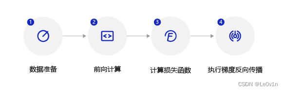
• Data preparation : convert a batch of data into nparrayformat first, and then into Tensorformat;
• Forward calculation : pour a batch of sample data into the network and calculate the output result;
• Calculate the loss function : take the forward calculation result and the real house price as input, and square_error_costcalculate the loss function value (Loss) through the loss function API.
• Back propagation : perform gradient back propagation backwardfunction, that is, calculate the gradient of each layer layer by layer from back to front, and update the parameters ( opt.stepfunction) according to the set optimization algorithm.

epochs = 100  # 总样本需要训练的轮次
batch_size = 10  # 每个 mini_batch 的样本数量

# 外层循环: 定义遍历数据集的次数，通过参数 epochs 设置
for epoch in range(epochs + 1):
    # 在每个 epoch 开始之前，将训练数据进行 Shuffle
    np.random.shuffle(training_data)
    
    # 将训练数据按照batch_size进行拆分
    mini_batches = [training_data[k: k + batch_size] for k in range(0, len(training_data), batch_size)]
    
    epoch_loss = []  # 记录损失
    
    # 内层循环： 负责整个数据集的一次遍历，采用分批次方式（mini-batch）。
    for iter_idx, mini_batch in enumerate(mini_batches):
        x = np.array(mini_batch[:, :-1])  # 训练样本
        y = np.array(mini_batch[:, -1:])  # 目标值

        # ndarray -> tensor
        inputs = paddle.to_tensor(x)
        targets = paddle.to_tensor(y)
        
        # infer
        preds = model(inputs)
        
        # calc losses
        losses = F.square_error_cost(input=preds, label=targets)
        
        # mean loss
        avg_loss = paddle.mean(losses, axis=0)
        epoch_loss.append(avg_loss.numpy())
            
        # 反向传播，计算每层参数的梯度值
        avg_loss.backward()

        # 让优化器更新参数
        optimizer.step()
        
        # 为下一个 epoch 清空当前梯度
        optimizer.clear_grad()
        
    # 打印损失
    print(f"Epoch: {
      
      epoch}\tLoss: {
      
      np.average(epoch_loss):.4f}")
    epoch_loss.clear()  # 清空历史损失

result:

W0805 03:36:18.712543 116394 gpu_resources.cc:119] Please NOTE: device: 0, GPU Compute Capability: 7.5, Driver API Version: 10.2, Runtime API Version: 10.2
W0805 03:36:18.715507 116394 gpu_resources.cc:149] device: 0, cuDNN Version: 8.2.
Epoch: 0        Loss: 0.2431
Epoch: 1        Loss: 0.0846
Epoch: 2        Loss: 0.0774
...
Epoch: 99       Loss: 0.0133
Epoch: 100      Loss: 0.0134

It is the same as PyTorch. Forward calculation, calculation loss and backpropagation gradient, each operation only requires 1 to 2 lines of code to implement. Flying Paddle has helped us automatically implement the process of reverse gradient calculation and parameter update, and we no longer need to write code one by one.

3.5 Save and test the model

3.5.1 Save model

Use the paddle.save API to save the current parameter data of the model model.state_dict()to a file for program calls for model prediction or verification.

# 保存模型
paddle.save(obj=model.state_dict(), path="LR_model.pdparams")
print(f"模型保存成功, 路径为: LR_model.pdparams")

Explanation : Why do we need to save the model instead of directly using the trained model for prediction?

In theory, predictions can be completed by directly using model instances, but in practical applications, training the model and using the model are often different scenarios . Model training usually uses a large number of offline servers (which do not provide online services to external corporate customers/users); model prediction is usually implemented using online servers that provide prediction services or the completed prediction model is embedded into mobile phones or other terminal devices. use. Therefore, the explanation method of "save the model first, then load the model" in this tutorial is more suitable for use in real scenarios.

3.5.2 Test model

Next, select a data sample to test the prediction effect of the model. The testing process is consistent with the process of using the model in the application scenario, and can be divided into the following three steps:

1. Configure machine resources for model predictions.
2. Load the trained model parameters LR_model.pdparamsinto the model instance. Completed by two statements:
   1. The first sentence is to read the model parameters from the file;
   2. The second sentence is to load the parameter content into the model.
   • After loading, you need to adjust the model's status to eval()(verification).
   • As mentioned above, the model in the training state needs to support both forward calculation and reverse conduction gradient. The implementation of the model is relatively bloated, while the model in the verification and prediction state only needs to support forward calculation. The implementation of the model is simpler and the performance is better. good.
3. Input the sample features to be predicted into the model and print the output prediction results.

We use load_one_examplethe function to extract a sample from the data set as a test sample. The specific implementation code is as follows.

def load_one_example(test_data):
    # 从已经加载的测试集中随机选择一条作为测试数据
    idx = np.random.randint(low=0, high=test_data.shape[0])
    one_data, label = test_data[idx, :-1], test_data[idx, -1:]
    
    # 修改该条数据的shape为 [1, 13]
    one_data = one_data.reshape([1, -1])
    
    return one_data, label


# 读取模型
model_dict = paddle.load("LR_model.pdparams")
model = Regression()
model.load_dict(state_dict=model_dict)
# 转换模型状态
model.eval()
    
# 读取单条测试数据
one_data, label = load_one_example(test_data=test_data)
one_data = paddle.to_tensor(one_data)
    
# 模型推理
pred = model(one_data)
    
# 对推理结果做反归一化处理
pred = pred * (max_values[-1] - min_values[-1]) + min_values[-1]
# 对真实标签做反归一化处理
label = label * (max_values[-1] - min_values[-1]) + min_values[-1]
    
print(F"推理结果为: {
      
      pred.numpy()}\t对应的真实值为: {
      
      label}")

result:

推理结果为: [[16.670935]]       对应的真实值为: [13.6]

By comparing the "model prediction value" and the "real house price", it can be seen that the prediction effect of the model is close to the real house price. House price prediction is only the simplest model, and you can get twice the result with half the effort if you use Flying Paddle to write it. Then for more complex models in industrial practice, the cost savings of using flying paddles are immeasurable. At the same time, Fei Paddle has optimized performance for many application scenarios and machine resources, and its functions and performance are far stronger than those of self-written models.

4. Grammatical differences between PaddlePaddle and PyTorch

4.1 Forward propagation: same

"""=============== PyTorch ==============="""
# 前向传播
loss = model(input_data, target)


"""=============== Paddle ==============="""
# 前向传播
loss = model(input_data, target)

4.2 Backpropagation: Same

"""=============== PyTorch ==============="""
loss.backward()


"""=============== Paddle ==============="""
# 反向传播
loss.backward()

4.3 Update parameters: same

"""=============== PyTorch ==============="""
# 定义优化器
optimizer = torch.optim.SGD(model.parameters(), lr=learning_rate)

# 更新参数
optimizer.step()


"""=============== Paddle ==============="""
# 定义优化器
optimizer = paddle.optimizer.SGD(learning_rate=learning_rate, parameters=model.parameters())

# 更新参数
optimizer.step()

4.4 Clear gradient: different

"""=============== PyTorch ==============="""
# 清空梯度
optimizer.zero_grad()


"""=============== Paddle ==============="""
# 清空梯度
optimizer.clear_gradients()

4.5 Model parameter file and model suffix: the same

"""=============== PyTorch ==============="""
# 保存模型参数
torch.save(model.state_dict(), "model.pt")  # 后缀一般是 .pt 或 .pth


"""=============== Paddle ==============="""
# 保存模型参数
paddle.save(model.state_dict(), "model.pdparams")  # 后缀一般是 .pdparams

4.6 Reading model: different

"""=============== PyTorch ==============="""
# 加载模型参数
model_state_dict = torch.load("model.pt")
model.load_state_dict(model_state_dict)


"""=============== Paddle ==============="""
# 加载模型参数
model_state_dict = paddle.load("model.pdparams")
model.set_state_dict(model_state_dict)

knowledge source

1. https://www.paddlepaddle.org.cn/tutorials/projectdetail/3520300
2. https://www.paddlepaddle.org.cn/tutorials/projectdetail/5836960
3. https://www.paddlepaddle.org.cn/tutorials/projectdetail/4309126