1. Generation of common distributed random numbers
1.1 Binomial distribution
In the Benoit experiment, the probability of an event A occurring is p, and the experiment is repeated n times. X represents the number of times A occurs in these n experiments. Then the probability distribution law (probability density) of the random variable
recorded as ![]()
thispdf(x,n,p) pdf('this',x,n,p)
Returns the density function value (probability distribution law value) of the binomial distribution at x with parameters n and p.
>> clear
>> x=1:30;y=binopdf(x,300,0.05);
plot(x,y,'b*')

binocdf(x,n,p) cdf('bino',x,n,p)
Returns the distribution function value of the binomial distribution at x with parameters n and p
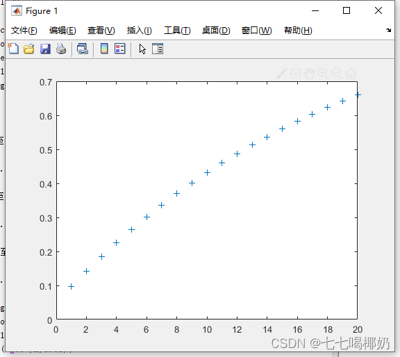
>> clear
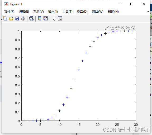
>> x=1:30;y=binocdf(x,300,0.05);
>> plot(x,y,'b+')
icdf('bino',q,n,p)
Inverse distribution calculation, returns the x value of the distribution function of the binomial distribution with parameters n and p when the probability is q.
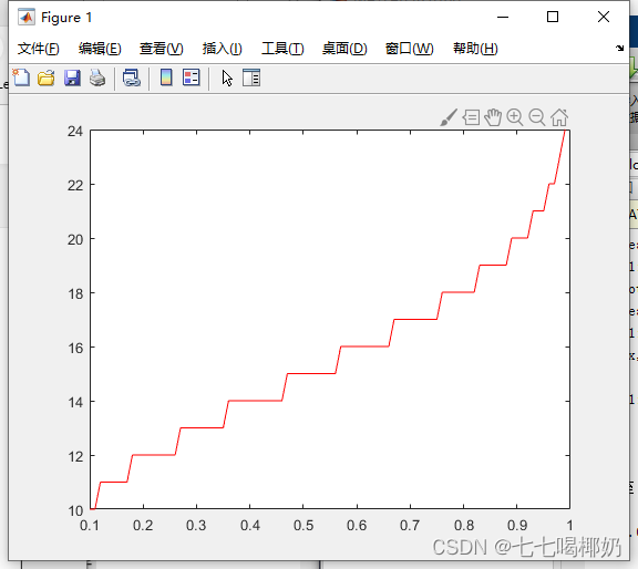
>> p=0.1:0.01:0.99;
>> x=icdf('bino',p,300,0.05);
>> plot(p,x,'r-')
R=binornd(n,p,m1,m2)
Generate random data in m1 rows and m2 columns obeying the binomial distribution with parameters n and p.
>> R=binornd(10,0.5,3,4)
R =
     0     6     5     5
     6     6     5     5
     4     5     5     4

>> A=binornd(10,0.2,3)
A =
     1     2     2
     1     3     1
     2     2     2
1.2 Poisson distribution
The Poisson distribution describes density problems: for example, the number of bacteria under the microscope X, the number of people infected with a certain disease in the unit population The number of pieces of information is X, etc.
The distribution law of X is (density function)
Denoted as ![]() where parameter λ represents the average value.
where parameter λ represents the average value.
boypdf(x,lambda) pdf('boy',x,lambda)
Returns the probability value of the Poisson distribution at x with parameter lambda.
>> clear
>> x=0:30;p=pdf('poiss',x,4);
>> plot(x,p,'b+')

boyscdf(x,lambda) cdf('boy',x,lambda)
Returns the distribution function value of the Poisson distribution at x with parameter lambda:
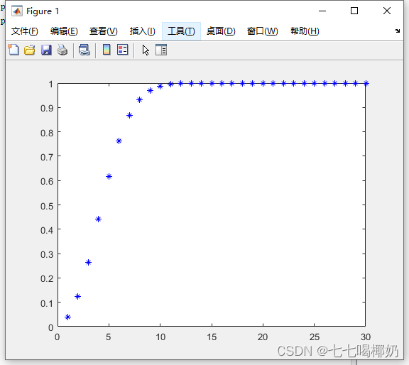
>> x=1:30;
>> p=cdf('poiss',x,5);
>> plot(x,p,'b*')
poissrnd(lambda,m1,m2)
Returns a random number in row m1 and column m2 that obeys the Poisson distribution with parameter lambda.
>> poissrnd(10,3,4)

ans =

    15    10     9     7
    14    10     7     9
    10     9    14    10
>> poissrnd(10,3)

ans =

    14    11     8
     8    11    13
     5    10    11
1.3 Geometric distribution
In a Bernoulli trial, the probability of success in each trial is p, and the probability of failure is q=1-p,0<p<1. The first successful trial occurs at the Xth time, then the distribution law of X is
geopdf(x,p)
Returns the probability value at x that obeys the geometric distribution with parameter p.
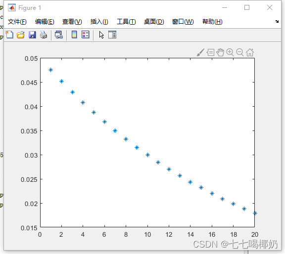
>> x=1:20;
>> p=geopdf(x,0.05);
>> plot(x,p,'*')
>> x=1:20;
>> p=cdf('geo',x,0.05);
>> plot(x,p,'+')
Returns the distribution function value
>> R=geornd(0.2,3,4)
R =
     0     0     5     0
     0     2     2     8
     9    10     0     0
>> R1=geornd(0.2,3)
R1 =
     0     8     1
     3     3     0
     0     0     1
1.4 Uniform distribution (discrete, equally likely distribution)

>> x=1:20;
>> p=unidpdf(x,20);f=unidcdf(x,20);
>> plot(x,p,'*',x,f,'+')

>> R=unidrnd(20,3,4)
R =
     1    14     8    15
    17    16    14     1
    19    15     4     6
>> R=unidrnd(20,3)
R =
     1    14     1
     2     7     9
    17    20     8
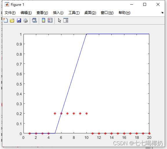
1.5 Uniform distribution (continuous type, etc. possible)

>> clear
>> x=1:20;p=unifpdf(x,5,10);
>> p1=unifcdf(x,5,10);
>> plot(x,p,'r*',x,p1,'b-')
>> R=unifrnd(5,10,3,4)
R =
    8.8276    7.4488    8.5468    8.3985
    8.9760    7.2279    8.7734    8.2755
    5.9344    8.2316    6.3801    5.8131

>> R1=unifrnd(5,10,3)
R1 =
    5.5950    6.7019    8.7563
    7.4918    7.9263    6.2755
    9.7987    6.1191    7.5298
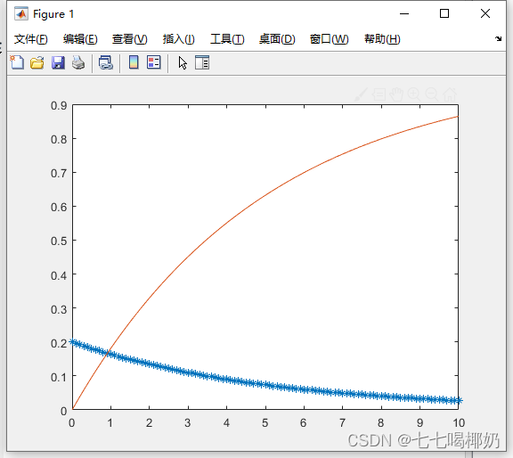
1.6 Exponential distribution (describing the "lifetime" problem)

>> x=0:0.1:10;
p=exppdf(x,5);
p1=expcdf(x,5);
plot(x,p,'*',x,p1,'-')
>> R=exprnd(5,3,4)
R =
    1.7900    3.0146    6.7835    1.0272
    0.5776    9.8799    0.8675    7.0627
    0.2078    9.5092    6.8466    0.3668

>> R1=exprnd(5,3)
R1 =
    5.2493    2.4222    0.9267
    8.1330    3.7402    2.6785
    6.9098    5.2255    2.9917
1.7 Normal distribution
![]()

clear
x=-10:0.1:15;
p1=normpdf(x,2,4);p2=normpdf(x,4,4);p3=normpdf(x,6,4);
plot(x,p1,'r-',x,p2,'b-',x,p3,'g-'),
gtext('mu=2'),gtext('mu=4'),gtext('mu=6')

clear
x=-10:0.1:15;
p1=normpdf(x,4,4);p2=normpdf(x,4,9);p3=normpdf(x,4,16);
plot(x,p1,'r-',x,p2,'b-',x,p3,'g-'),
gtext('sig=2'),gtext('sig=3'),gtext('sig=4')

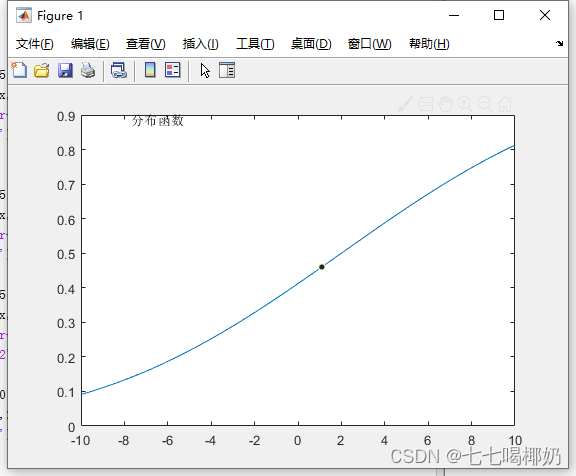
>> clear
>> x=-10:0.1:10;
>> p=normcdf(x,2,9);
>> plot(x,p,'-'),gtext('分布函数')
>> p=[0.01,0.05,0.1,0.9,0.05,0.975,0.9972];
>> x=icdf('norm',p,0,1)
x =
-2.3263 -1.6449 -1.2816
1.2816 -1.6449 1.96 2.7703
x=icdf('norm',p,0,1)
Calculate the inverse function value of the distribution function of the standard normal distribution, that is, return the corresponding quantile if the probability is known.
Generate normally distributed random numbers
>> R=normrnd(0,1,3,4)
R =
    1.5877    0.8351   -1.1658    0.7223
   -0.8045   -0.2437   -1.1480    2.5855
    0.6966    0.2157    0.1049   -0.6669
>> R1=normrnd(0,1,3)
R1 =
    0.1873   -0.4390   -0.8880
   -0.0825   -1.7947    0.1001
   -1.9330    0.8404   -0.5445