Power spectrum estimation of periodic and random signals is probably one of the most important application areas of digital signal processing (DSP).
Spectral analysis encompasses a wide and potentially unlimited variety of measurement methods, so the purpose of this text is to provide a brief and basic introduction to the concept of power spectrum estimation and its Matlab implementation.
1. Basic content
1. Spectrum
A spectrum is a relationship, usually represented by a plot of the magnitude or relative value of some parameter versus frequency . Every physical phenomenon, whether electromagnetic, thermal, mechanical, hydraulic, or any other system, has a unique spectrum.
In electronics, these phenomena are dealt with using signals, represented by fixed or varying voltages, currents, and powers. These quantities are usually described in the time domain. For each time function f(t) , an equivalent frequency domain function F(w) can be found , which specifically describes the frequency component content required to generate f(t). (spectrum) .
The subject of Fourier analysis and Fourier transform is the study of the relationship between the time domain and the corresponding frequency domain representation .
The forward Fourier transform of function x(t), the definition from time domain to frequency domain:
inverse Fourier transform, the definition of frequency domain to time domain:
2. Energy and power
The time domain and frequency domain signal functions are connected by using Fourier transform. The focus here is mainly on analyzing signal power and energy .
Parseval's theorem Theorem Parseval's theorem connects the representation of energy w(t) in the time domain and frequency domain through the following expression.
*Parseval's theorem shows that the energy of the signal is equal in the time domain and frequency domain.
*where f(t) is an arbitrary signal that changes with time, and F(f) is the equivalent Fourier transform representation in the frequency domain.
This theorem simply states that the total energy of a signal f(t) is equal to the area under the square of its Fourier transform amplitude . |F(f)|^2 is often called energy density, spectral density or power spectral density function, |F(f)|^2 df describes the differential frequency band from f to f+dF Contains signal energy density.
In many electrical engineering applications, instantaneous signal power is required, which is usually assumed to be equal to the square of the signal amplitude, i.e., f^2*(t).
For convenience, assume that the signal in the system passes through a 1 ohm resistor. For example, if f(t) is a voltage (current) signal applied to the system resistance R, its true instantaneous power is expressed as [f(t)^2]/R (or for current [f(t)^2] R). Therefore, f^2*(t) is the real power only when R is 1 ohm.
For periodic signals , the average power Pavg in the time region t1-t2 can be defined by integrating [f(t)]^2 from t1 to t2, and then dividing by t2-t1 to obtain the average value:
where T is the period of the signal.
Energy can be expressed in terms of power P(t):
Power is the rate of change of energy over time:
|F(f)|^2 and P(t) are often called energy density, spectral density or power spectral density function PSD . Furthermore, PSD can be interpreted as the average power associated with a 1Hz bandwidth centered at fHz.
3. Random signal
The use of Fourier transform to analyze linear systems is widespread and can easily handle periodic signals. But for random signals, is it possible to perform Fourier transform directly like periodic signals? With some modifications, it still works. And the modified method provides essentially the same advantages in processing random signals as in processing non-random signals.
*Random signal (stationary/non-stationary): uncertain, unpredictable in amplitude, non-periodic, but often subject to certain statistical characteristics.
2. Classic power spectrum estimation method
The traditional Fourier analysis method used in classic power spectrum estimation is mainly divided into two types: autocorrelation method (indirect method) and periodogram method (direct method) .
How to evaluate the quality of power spectrum estimation? ——Resolution and variance
*Resolution: The smallest adjacent frequency component that can be distinguished on the power spectrum. The higher the resolution, the clearer the frequency components of the signal we observe;
*Variance: The size of the variance reflects the volatility of the power spectrum. If the variance is too large and the volatility of the power spectrum is large, it is easy to cause useful frequency components to be overwhelmed by noise. Therefore, for the power spectrum we hope to obtain, the higher the resolution, the better, and the smaller the variance, the better.
1. Autocorrelation method
In 1949, Turkey proposed the autocorrelation method for spectral estimation of finite-length data based on the Wiener-Khintchine theorem, that is, using finite-length data to estimate the autocorrelation function , and then obtaining the Fourier transform of the autocorrelation function to obtain an estimate of the spectrum.
In 1958, Blackman and Tukey discussed the autocorrelation spectrum estimation method in their publication on classical spectral estimation, so the autocorrelation method is also called the BT method . Proceed as follows:
(1) The autocorrelation function R(m) is estimated from a limited number of observed values x(0), x(1),...x(n-1) of the signal;
(2) Perform Fourier transformation on R(m) to obtain the power spectrum;
*The Wiener-Khintchine theorem states that the correlation function of a random signal and its power spectrum are a pair of Fourier transforms.
The power spectrum obtained by the BT method with the number of data points N being 256, 512 and 1024 is shown in the figure, and the variance values are shown in the table.

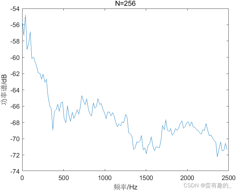
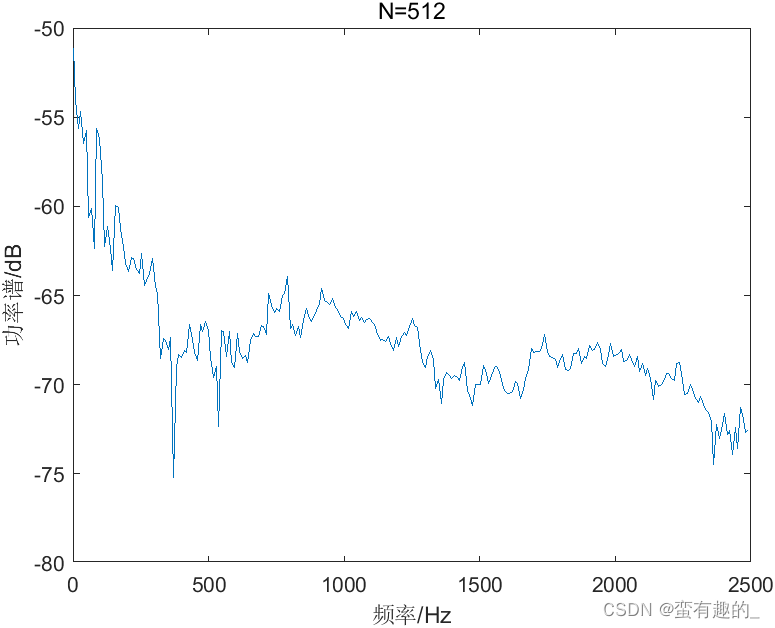
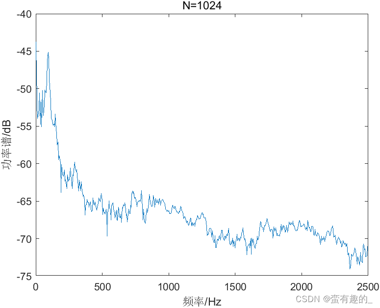
| N | 256 | 512 | 1024 |
| variance | 11.83 | 12.00 | 23.72 |
It is found from the results that as N increases, the resolution increases and the variance becomes larger. The BT method does not resolve the contradiction between resolution and variance. The code is as follows (N=1024):
filename = 'sample.wav';%读取音频文件
[xn, Fs] = audioread(filename);%得到采样频率Fs和音频数据s
nfft=1024;
cxn=xcorr(xn,'unbiased'); %计算序列的自相关函数
CX_fft=fft(cxn,nfft);
Pxx=abs(CX_fft);
index=0:round(nfft/2-1);
f=index*Fs/nfft;%计算频率范围
plot_Pxx=10*log10(Pxx(index+1));
plot(f,plot_Pxx);
xlabel('频率/Hz');
ylabel('功率谱/dB');
title('N=1024');
A = std(plot_Pxx)^2;
2. Periodogram method
In 1899, Schuster first proposed the periodogram method , also known as the direct method . Take a limited number of observation values x(0), x(1),...x(N-1) of the stationary random signal X(n) to estimate the power spectrum S(w). Proceed as follows:
(1) Cut an N-long segment from the random signal X(n) and treat it as a signal with limited energy;
(2) Perform Fourier transform on the sequence to obtain the spectrum;
(3) Take the square of its amplitude value and divide it by N.
*This is the earliest formulation of classical spectrum estimation. This method is still used today, except that now Fast Fourier Transform (FFT) is used to calculate the Discrete Fourier Transform (DFT), and the square amplitude of the DFT is used as the signal. A measure of medium power.
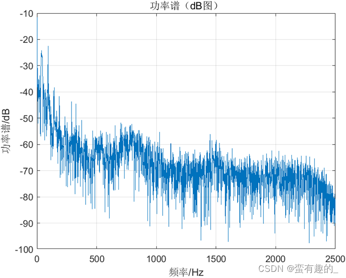
When the number of data points N is 1280, 2560 and 5120 respectively, the obtained power spectra are as shown in the figure. The resolution can be seen intuitively through the power spectrum diagram, and the variance value is shown in the table.
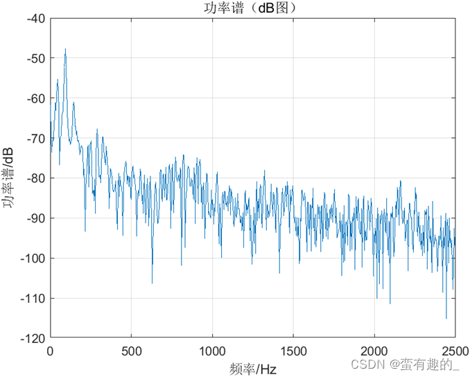

| N | 1280 | 2560 | 5120 |
| variance | 7.23e-13 | 2.48e-10 | 1.33e-6 |
Through the above results, the power spectrum obtained by the periodogram method has a larger resolution and a larger variance as the number of data points N increases. code show as below:
filename = 'sample.wav';%读取音频文件
[xn, Fs] = audioread(filename);%得到采样频率Fs和音频数据s
N=1280;%数据点选取
Nfft=N;
n=0:N-1;&数据点序列
xn = xn(1:N);%截取信号
P=10*log10(abs(fft(xn,Nfft).^2)/N);%傅里叶变换振幅谱平方的平均值,并转化为dB
f=(0:length(P)-1)*Fs/length(P);%频率序列
figure;
plot(f(1:N/2),P(1:N/2));
grid on;
title('功率谱(dB图)');
ylabel('功率谱/dB');
xlabel('频率/Hz');
3. Common improvement cycle chart methods
Average period chart method
As the number of data points N increases, the power spectrum obtained by the periodogram method becomes larger in resolution and variance. It contradicts our expectation of "large resolution and small variance".
To improve this performance. MSBartlett proposed the average periodogram method, which divides the signal sequence x(n) into several non-overlapping segments. The power spectrum is estimated for each small segment of the signal sequence, and then averaged as the power spectrum estimate of the entire sequence x(n). Proceed as follows:
(1) Divide the signal x(n) into non-overlapping segments (the number of segments is L);
(2) Estimating the power spectrum of each small segment signal sequence;
(3) Take the average as the power spectrum estimate of the entire sequence x(n).
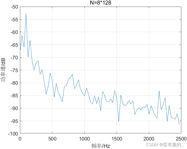
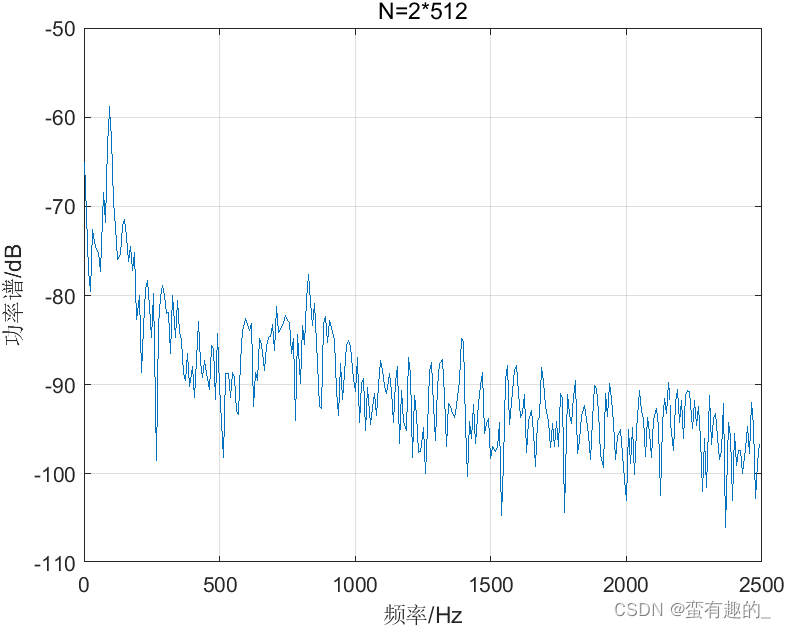
When the number of data points N is 1280 and the number of segments is 8, 4, and 2 respectively, the obtained power spectra of the average power spectrum are as shown in the figure.

| L | 8 | 4 | 2 |
| variance | 3.67e-13 | 5.42e-15 | 7.45e-15 |
The appropriate resolution and variance can be determined by selecting the number of data points and the number of segments L.
code show as below:
filename = 'sample.wav';%读取音频文件
[xn, Fs] = audioread(filename);%得到采样频率Fs和音频数据s
Nsec=640;%FFT所用的数据长度
Pxx1=abs(fft(xn(1:640),Nsec).^2)/Nsec; %第一段功率谱
Pxx2=abs(fft(xn(641:1280),Nsec).^2)/Nsec;%第二段功率谱
Pxx=10*log10((Pxx1+Pxx2)/2);%Fourier振幅谱平方的平均值,并转化为dB
a11=std((Pxx1+Pxx2)/2)^2;
f=(0:length(Pxx)-1)*Fs/length(Pxx);%给出频率序列
figure;
plot(f(1:Nsec/2),Pxx(1:Nsec/2));%绘制功率谱曲线
xlabel('频率/Hz');
ylabel('功率谱/dB');
title('N=2*512');
grid on;
Nsec=320;%数据的长度和FFT所用的数据长度
Pxx1=abs(fft(xn(1:320),Nsec).^2)/Nsec; %第一段功率谱
Pxx2=abs(fft(xn(321:640),Nsec).^2)/Nsec;%第二段功率谱
Pxx3=abs(fft(xn(641:960),Nsec).^2)/Nsec;%第三段功率谱
Pxx4=abs(fft(xn(961:1280),Nsec).^2)/Nsec;%第四段功率谱
Pxx=10*log10((Pxx1+Pxx2+Pxx3+Pxx4)/4);%Fourier振幅谱平方的平均值,并转化为dB
a12=std((Pxx1+Pxx2+Pxx3+Pxx4)/4)^2;
f=(0:length(Pxx)-1)*Fs/length(Pxx);%给出频率序列
figure;
plot(f(1:Nsec/2),Pxx(1:Nsec/2));%绘制功率谱曲线
xlabel('频率/Hz');
ylabel('功率谱/dB');
title('N=4*256');
grid on;

Nsec=160;%数据的长度和FFT所用的数据长度
Pxx1=abs(fft(xn(1:160),Nsec).^2)/Nsec; %第一段功率谱
Pxx2=abs(fft(xn(161:320),Nsec).^2)/Nsec;%第二段功率谱
Pxx3=abs(fft(xn(321:480),Nsec).^2)/Nsec;%第三段功率谱
Pxx4=abs(fft(xn(481:640),Nsec).^2)/Nsec;%第四段功率谱
Pxx5=abs(fft(xn(641:800),Nsec).^2)/Nsec; %第五段功率谱
Pxx6=abs(fft(xn(801:960),Nsec).^2)/Nsec;%第六段功率谱
Pxx7=abs(fft(xn(961:1120),Nsec).^2)/Nsec;%第七段功率谱
Pxx8=abs(fft(xn(1121:1280),Nsec).^2)/Nsec;%第八段功率谱
Pxx=10*log10((Pxx1+Pxx2+Pxx3+Pxx4+Pxx5+Pxx6+Pxx7+Pxx8)/8);%Fourier振幅谱平方的平均值,并转化为dB
a13=std((Pxx1+Pxx2+Pxx3+Pxx4+Pxx5+Pxx6+Pxx7+Pxx8)/8)^2;

f=(0:length(Pxx)-1)*Fs/length(Pxx);%给出频率序列
figure;
plot(f(1:Nsec/2),Pxx(1:Nsec/2));%绘制功率谱曲线
xlabel('频率/Hz');
ylabel('功率谱/dB');
title('N=8*128');
grid on;
When the number of observation sample sequence data N is fixed, to reduce the variance, the number of segments L needs to be increased. When N is not large, the segment length M takes a small value, and the power spectrum resolution is reduced to a lower level. If the number of segments L is fixed, increasing the resolution requires a segment length M, and a longer detection data sequence needs to be collected. In practice, the length of the detection sample sequence is insufficient.
modified mean periodogram method
The length of the actual detection sample sequence mentioned in the above method is limited. For the existing data length N, if more segments can be divided, a smaller variance will be obtained. Allow overlap between data segments to obtain more segments. The simplest way to select the overlap length between segments is to take half of the segment length M.
PD Welch further improved on the Bartlett method and proposed a method that combines windowing processing with segmented averaging, which uses signal overlapping segmentation, windowing, FFT and other techniques to calculate the power spectrum.
The process of data interception is equivalent to adding a rectangular window to the data. The larger side lobes of the rectangular window will cause "spectrum leakage". The window functions adopted during segmentation are more diverse (triangular window, Hamming window, etc.) to reduce the impact of truncated data (adding rectangular windows) window functions.
Proceed as follows:
(1) First perform overlapping segmentation on the signal x(n). For example, according to 2:1 overlapping segmentation, that is, the previous segment of the signal and the subsequent segment of the signal overlap by 1/2;
(2) Then use a non-rectangular window to preprocess each small segment of the signal sequence, and then use the aforementioned segmented average periodogram method to estimate the power spectrum of the entire signal sequence x(n).
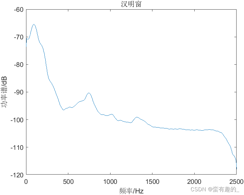
*Compared with the periodogram method, the Welch method can greatly improve the smoothness of the spectral curve and improve the resolving power of spectral estimation.
When selecting different window functions (rectangular window, Hamming window, blackman window), the pwelch function is used for spectrum estimation. The result is shown in the figure:


code show as below:
filename = 'sample.wav';%读取音频文件
[xn, Fs] = audioread(filename);%得到采样频率Fs和音频数据s
nfft=xn;
window=boxcar(100); %矩形窗
window1=hamming(100); %海明窗
window2=blackman(100); %blackman窗
noverlap=50; %重叠
range='onesided'; %频率间隔为[0 Fs/2],只计算一半的频率
[Pxx,f]=pwelch(xn,window,noverlap,nfft,Fs,range);
[Pxx1,f1]=pwelch(xn,window1,noverlap,nfft,Fs,range);
[Pxx2,f2]=pwelch(xn,window2,noverlap,nfft,Fs,range);
plot_Pxx=10*log10(Pxx);
plot_Pxx1=10*log10(Pxx1);
plot_Pxx2=10*log10(Pxx2);

figure
plot(f,plot_Pxx);title('矩形窗');

figure
plot(f1,plot_Pxx1);title('汉明窗');

figure
plot(f2,plot_Pxx2);title('blackman窗');
Reference: Internet content