Table of contents
1. Create a table and insert data
3. GROUP BY aggregate function
3.4 Use the GROUP BY function to find missing values
3.5 Use the GROUP BY function to measure data quality
4.1 Basic knowledge of window functions
4.1.1 OVER does not contain keywords
4.1.2 Using PARTITION BY alone
4.1.4 Using PARTITION BY and ORDER BY simultaneously
1. Create a table and insert data
DROP TABLE IF EXISTS 学生;
create table 学生
(
    student_id INT PRIMARY KEY,
    gender TEXT,
    city TEXT,
    a_score FLOAT(2),
    b_score FLOAT(2),
    weight FLOAT(2)
)engine=innodb;

INSERT INTO 学生 VALUES
(001,'female','xiameng',90.6,110.87,50.34),
(002,'male','guangzhou',93.6,116.87,48.6),
(003,NULL,'guangzhou',90.64,107.06,60.34),
(004,'female','guangzhou',80.6,103.87,45.0),
(005,NULL,'xiameng',NULL,98.8,50.34),
(006,'female','guangzhou',90.6,113.87,50.34),
(007,'female','xiameng',NULL,110.02,50.34),
(008,'male','wuhan',90.6,90.87,50.34),
(010,'male','guangzhou',90.6,98.87,48.6),
(011,'female','xiameng',90.6,96.87,48.6),
(012,'male','xiameng',90.6,87.17,50.34),
(013,NULL,'xiameng',90.6,80.87,48.6),
(014,'female','guangzhou',90.6,103.87,50.34),
(015,NULL,'xiameng',90.6,98.87,50.34),
(016,'female','wuhan',NULL,110.87,50.34),
(017,'female','guangzhou',90.6,98.87,50.34),
(018,'female','xiameng',90.6,96.87,50.34),
(019,'female','guangzhou',90.6,110.95,48.6),
(020,'female','wuhan',90.6,110.87,50.34),
(021,NULL,'guangzhou',NULL,110.87,50.34),
(022,'female','guangzhou',90.6,110.87,50.34),
(023,NULL,'wuhan',90.6,110.87,50.34),
(024,'female','guangzhou',90.6,110.87,50.34),
(025,'female','guangzhou',90.6,110.87,48.6),
(026,'male','guangzhou',NULL,110.87,50.34),
(027,'female','wuhan',90.6,110.87,50.34),
(028,'female','guangzhou',90.6,110.87,48.6),
(029,'female','xiameng',90.6,110.87,48.6),
(030,'male','guangzhou',90.6,110.87,45.0),
(031,'female','xiameng',NULL,110.87,50.34),
(032,'female','guangzhou',90.6,110.87,50.34),
(033,NULL,'guangzhou',NULL,96.5,50.34),
(034,'female','wuhan',90.6,96.5,45.0),
(035,'male','guangzhou',90.6,110.87,50.34),
(036,'female','wuhan',90.6,96.5,50.34),
(037,'female','guangzhou',90.6,110.87,50.34),
(038,'male','wuhan',90.6,110.87,50.34),
(039,'female','guangzhou',90.6,110.87,50.34),
(040,'male','xiameng',NULL,110.87,50.34),
(041,'female','wuhan',90.6,107.06,50.34),
(042,NULL,'guangzhou',NULL,110.87,50.34),
(043,'female','guangzhou',90.6,110.87,45.0),
(044,'male','wuhan',90.6,110.87,50.34),
(045,'female','xiameng',90.6,110.87,50.34),
(046,'female','guangzhou',90.6,107.06,50.34),
(047,'male','guangzhou',90.6,110.87,50.34),
(048,'female','guangzhou',90.6,96.5,45.0),
(049,NULL,'wuhan',NULL,107.06,50.34),
(050,NULL,'wuhan',90.6,110.87,50.34),
(051,NULL,'wuhan',NULL,110.87,50.34),
(052,NULL,'guangzhou',90.6,96.5,50.34),
(053,'female','guangzhou',90.6,110.87,50.34),
(054,NULL,'wuhan',90.6,110.87,48.6),
(055,'female','xiameng',90.6,110.87,50.34),
(056,NULL,'xiameng',90.6,107.06,45.0),
(057,'male','guangzhou',90.6,96.5,50.34),
(058,NULL,'guangzhou',90.6,110.87,50.34),
(059,NULL,'wuhan',NULL,110.87,48.6),
(060,'female','wuhan',NULL,110.87,48.6);
2. Common aggregate functions
| function | explain |
| COUNT(columnX) | Count the number of rows containing non-null values in columnX |
| COUNT(*) | Count the number of rows in the output table |
| MIN(columnX) | Returns the minimum value in columnX. For text classes, returns the value that appears first in alphabetical order |
| MAX(columnX) | Returns the maximum value in columnX |
| SUM(columnX) | Returns the sum of all values in columnX |
| AVG(columnX) | Returns the average of all values in columnX |
| STDDEV(columnX) | Returns the sample standard deviation of all values in columnX |
| VAR(columnX) | Returns the sample variance of all values in columnX |
| REGR_SLOPE(columnX,columnY) | Returns the slope of linear regression when columnX is used as the dependent variable and columnY is used as the independent variable. |
| REGR_INTERCEPT(columnX,columnY) | Returns the intercept of linear regression when columnX is used as the dependent variable and columnY is used as the independent variable. |
| CORR(columnX,columnY) | Returns the Pearson correlation coefficient between columnX and columnY in the data |
SELECT COUNT(DISTINCT city) FROM 学生;
SELECT COUNT(*) FROM 学生 WHERE city='xiameng';
SELECT COUNT(*)/2 FROM 学生 WHERE city='xiameng'; 

SELECT MIN(b_score),MAX(b_score),AVG(b_score),STDDEV(b_score) FROM 学生;
3. GROUP BY aggregate function
3.1 GROUP BY child clause
GROUP BY is a clause that divides the rows of a dataset into multiple groups based on some key specified in the GROUP BY clause and then applies an aggregate function to all in a single group to produce a single number.
Use GROUP BY to query how many students there are in each city
SELECT city,COUNT(*) FROM 学生 GROUP BY city ORDER BY city;
SELECT city,COUNT(*) FROM 学生 WHERE gender='female' GROUP BY city ORDER BY COUNT(*)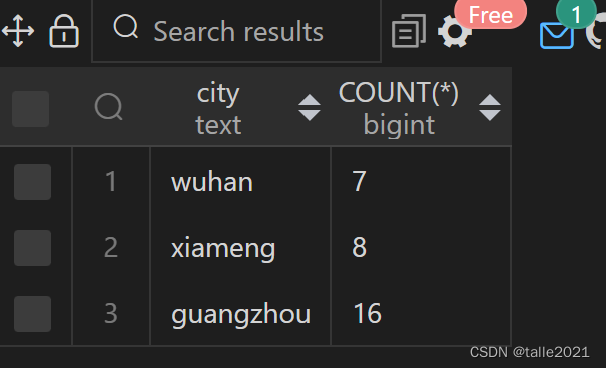
3.2 Multi-column GROUP BY
Use GROUP BY to query how many male and female students there are in each city
SELECT city,gender,count(*) FROM 学生 GROUP BY city,gender ORDER BY city,gender;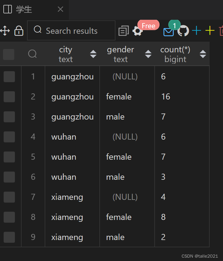
3.3 HAVING clause
The HAVING clause is similar to the WHERE clause, except that it is specially designed for GROUP BY queries.
SELECT city,gender,count(*) FROM 学生 GROUP BY city,gender HAVING gender IS NOT NULL ORDER BY city,gender;
3.4 Use the GROUP BY function to find missing values
To determine whether a column has missing values, you can use a modified CASE WHEN statement with the SUM and COUNT functions to determine the percentage of missing data.
Based on the query results, if the proportion of missing data is very small (<1%), you can consider filtering or deleting the missing data from the analysis. If a certain percentage of data is missing (<20%), you can consider filling in the missing data using typical values (mean, mode, etc.). If more than 20% of the data is missing, consider removing the column because there is not enough accurate data to draw accurate conclusions based on the values in the column.
Query the proportion of missing values in the a_score column:
SELECT SUM(CASE
    WHEN a_score is NULL
    THEN 1
    ELSE 0
END)/COUNT(*) AS missing_score FROM 学生;
3.5 Use the GROUP BY function to measure data quality
If you want to determine if each value in a column is unique. Although in most cases this can be solved by setting the column of the primary key constraint, this is not always possible.
For example, verify whether the value contained in the student_id column in the student table is unique:
SELECT COUNT(DISTINCT student_id)=COUNT(*) AS equal_id FROM 学生;
SELECT COUNT(DISTINCT city)=COUNT(*) AS equal_city FROM 学生; 

If the query result returns 1, then each row of the column has a unique value; otherwise, there is at least one duplicate value.
4. Window functions
Aggregation functions allow analysts to take many rows and convert those rows into a number. For example, the COUNT function can get the number of rows in a table and return the number of rows. However, sometimes we want to be able to calculate multiple rows but still retain all the rows after calculation. Window functions can take multiple rows of data and process them but still retain all the information.
4.1 Basic knowledge of window functions
Basic syntax of window functions:
SELECT {columns},{window_func} OVER (PARTITION BY {partition_key} ORDER BY {order_key}) FROM tabel;{columns} are the columns to be retrieved from the query table
{window_func} is the window function to be used
{partition_key} is the column to be partitioned
{order_key} is the column to be sorted
4.1.1 OVER does not contain keywords
SELECT student_id,gender,city,COUNT(*) OVER() AS total_student FROM 学生 ORDER BY student_id;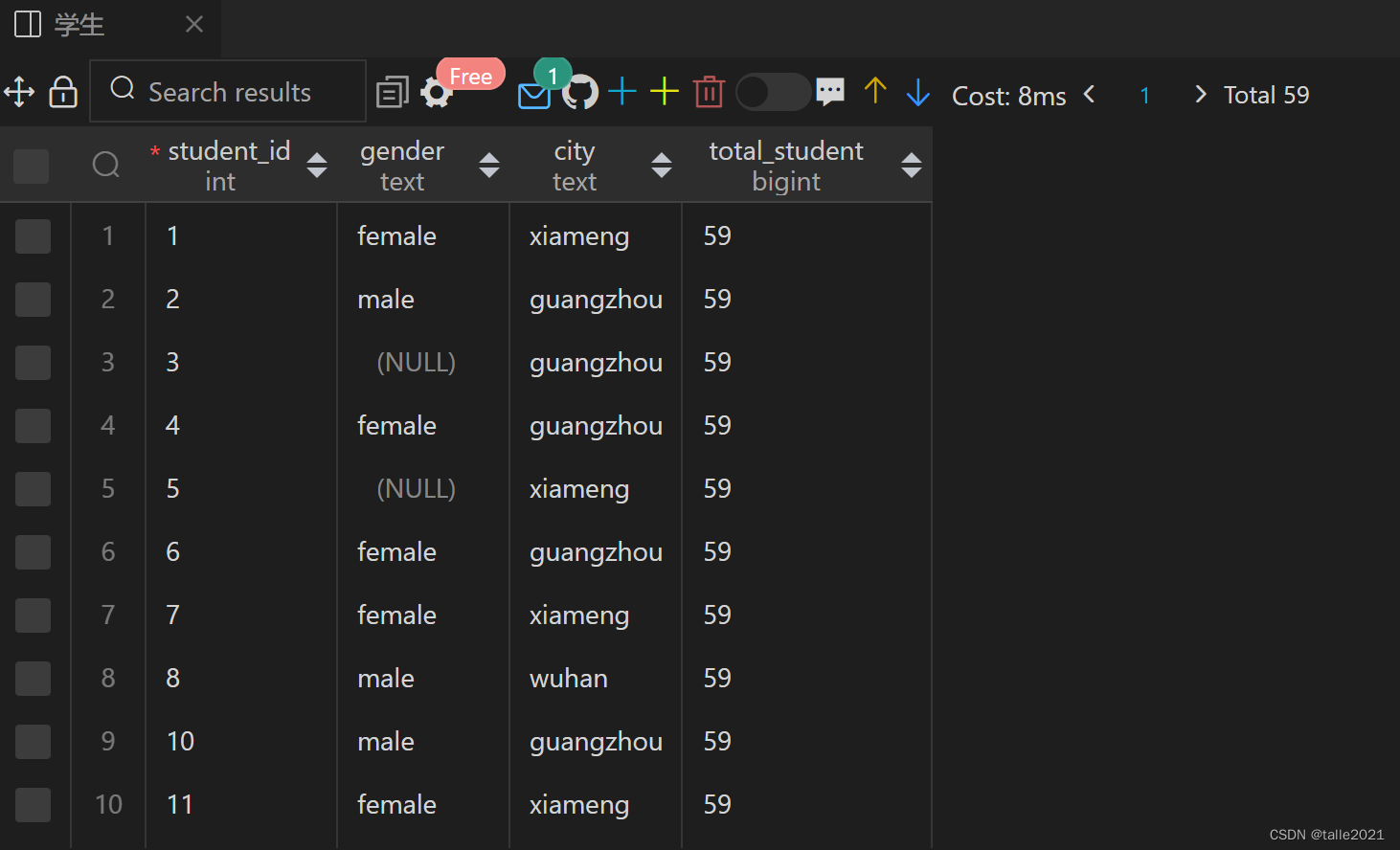
The result returns all rows and COUNT(*).
4.1.2 Using PARTITION BY alone
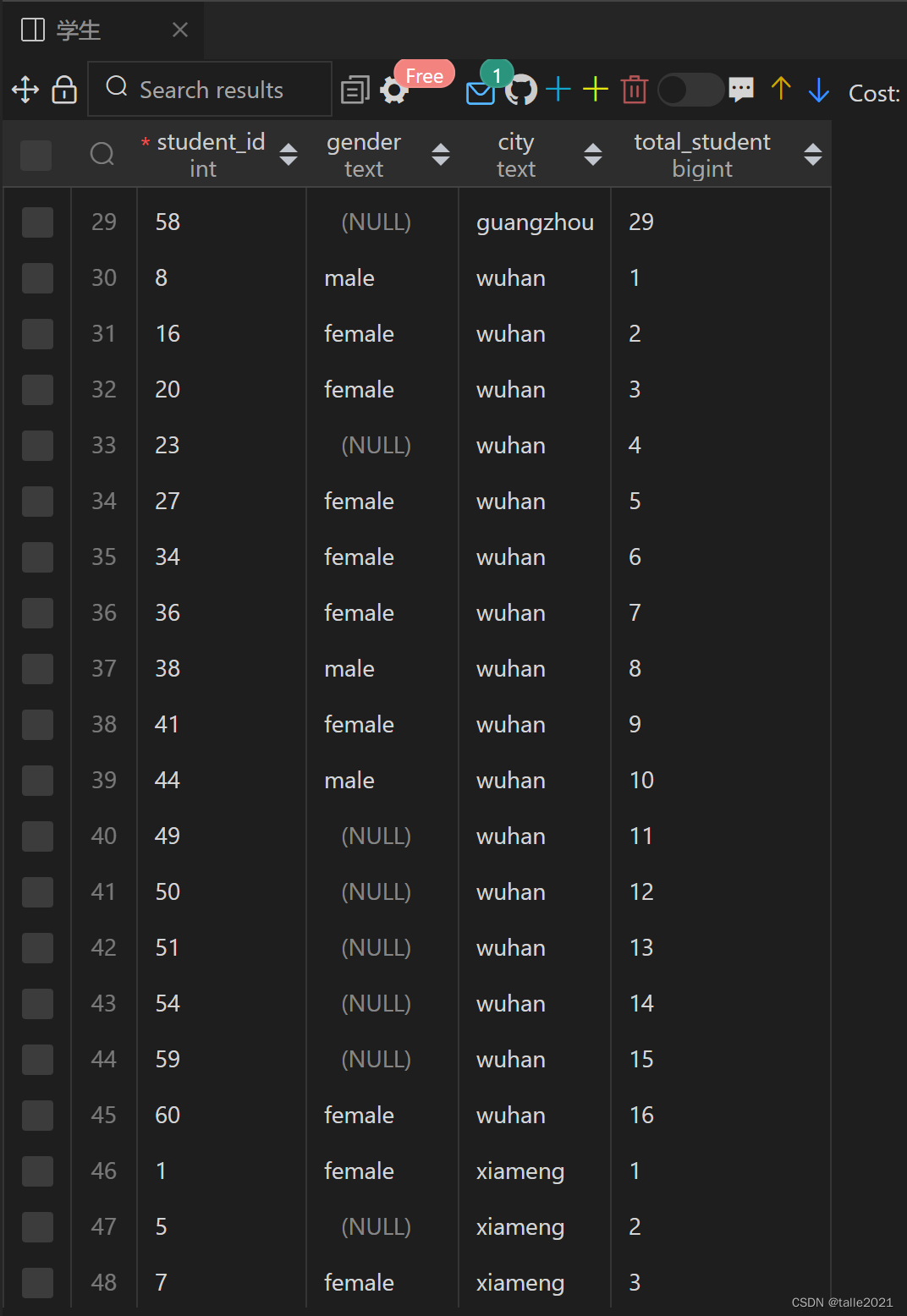
SELECT student_id,gender,city,COUNT(*) OVER(PARTITION BY city) AS total_student FROM 学生 ORDER BY student_id;
After using partition by to divide into 3 groups, the value of total_student count is now changed to one of 3 values, that is, the number of students corresponding to each city.
4.1.3 Using ORDER BY alone
SELECT student_id,gender,city,COUNT(*) OVER(ORDER BY student_id) AS total_student FROM 学生 ORDER BY student_id
The count at this time is similar to the accumulation of the total number of students, which is the origin of the name "window" in the window function. When using window functions, the query creates a "window" over the table it counts. PARTITION BY works similar to GROUP BY, dividing the data set into multiple groups, and for each group, a window is created. If ORDER BY is not specified, the default window is the entire group.
However, when ORDER BY is specified, the rows in the group are sorted according to it, and for each row, a window is created and the row count is applied over that window.
As shown in the table above, the window in row 1 contains one row and returns a count of 1, the window in row 2 contains two rows and returns a count of 2, and the window in row 3 contains three rows and returns a count of 3.
4.1.4 Using PARTITION BY and ORDER BY simultaneously
SELECT student_id,gender,city,COUNT(*) OVER(PARTITION BY city ORDER BY student_id) AS total_student FROM 学生 ORDER BY city;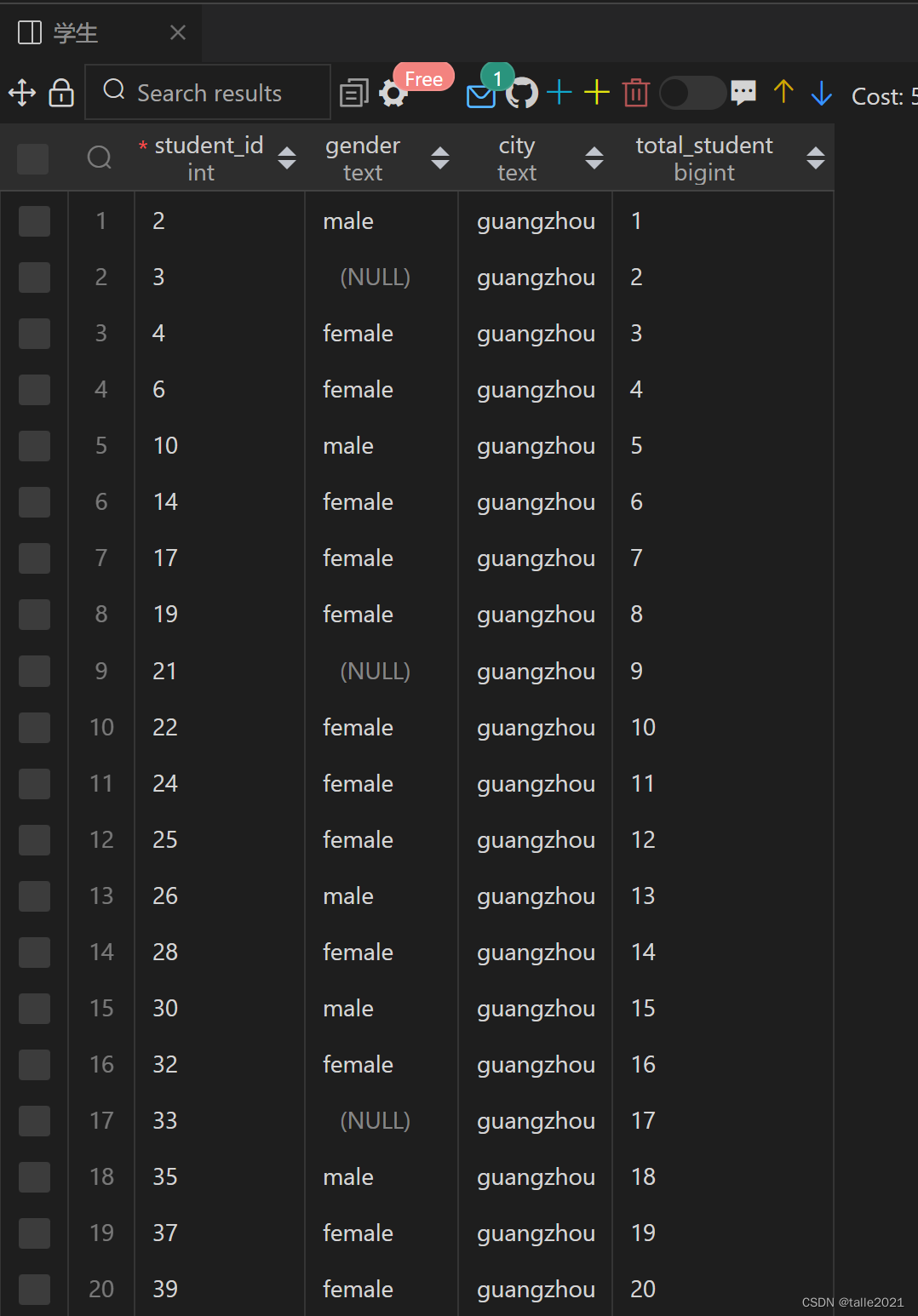
This query first divides the data set into 3 groups by city based on PARTITION BY city. Each group has its own set of windows, and then counts each group separately.
4.2 WINDOW keyword
For some functions, if you need to perform different function calculations on the same window, for example: query the cumulative total number of students in each city and the cumulative total number of students in each city whose gender is unknown:
SELECT student_id,city,gender,
COUNT(*) OVER (PARTITION BY city ORDER BY student_id) AS total_student,
SUM(CASE
    WHEN gender IS NULL THEN  1
    ELSE  0
END) OVER (PARTITION BY city ORDER BY student_id) AS total_gender
FROM 学生 ORDER BY student_id;
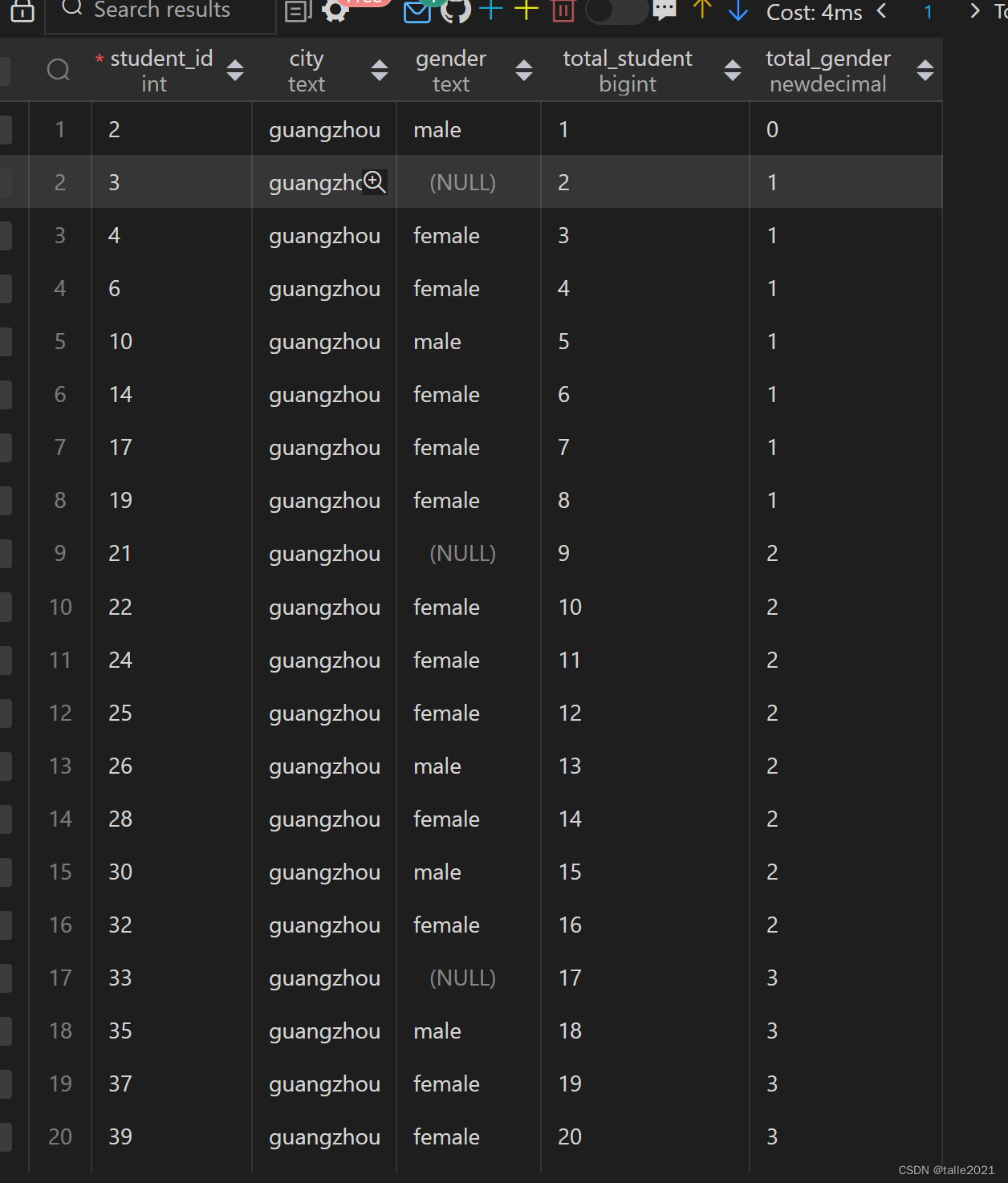
This query first divides the data set into 3 groups by city based on PARTITION BY city. Each group has its own set of windows. For each group, for every additional student, the total_student value increases by 1; every time a "NULL" appears in the gender column " value, add 1 to the total_gender column value.
Although this query provides the desired results, it is cumbersome to write and can be simplified using the WINDOW clause:
SELECT student_id,city,gender,
COUNT(*) OVER w AS total_student,
SUM(CASE
    WHEN gender IS NULL THEN  1
    ELSE  0
END) OVER w AS total_gender
FROM 学生
WINDOW w AS (PARTITION BY city ORDER BY student_id)
ORDER BY city;