Table of contents
4. Summary discussion and exploration
Problem Description
For JPEG's classic steganography algorithms Jsteg and F5 algorithms, secret data can be written in JPEG images. This experiment wants to determine the type of JPEG image (original image and steganographic image) through different JPEG steganalysis methods. In order to distinguish the JPEG encrypted image from the original image, the two JPEG steganalysis methods are analyzed and tested.
1. Program functions
1. Program function description (task1-task5 are five main programs, and the rest are auxiliary programs)
task1: Verify the approximation of the block feature value of the original compressed image and the block feature value of the reference image of the encrypted image. The block feature value of the encrypted image is greater than the block feature value of its reference image, but at the same time it is found that the original compression The block feature value of the image is also larger than the block feature value of its reference image;
task2: Use 20 standard images for testing. Under different quality factors QF, compare the block feature values of the encrypted image with the block feature values of its reference image and the block feature values of the original compressed image with its reference image. , which proves that the difference between the block feature values of the encrypted image and its reference image is larger than the difference between the block feature values of the original compressed image and its reference image;
task3: Use 84 standard images for testing. Under the quality factor QF=70, the block feature values of the encrypted image and its reference image and the block feature values of the original compressed image and its reference image are determined. Comparison, find an obvious limit value by comparing the pictures, and use this limit value to identify the image type of 168 images (84 images with confidentiality and 84 images without confidentiality), and the discrimination accuracy is 84.39%;
task4: Verify the approximation of the histogram of the original compressed image and the DCT coefficient histogram of the reference image. The DCT coefficient histogram of the encrypted image is relatively high compared to the DCT coefficient histogram of its reference image. At the same time, it is found that the DCT coefficient histogram of the original image is The DCT coefficient histogram also has relatively high characteristics compared to the DCT coefficient histogram of its reference image. However, it is found that in certain circumstances, the DCT coefficient of the encrypted image is 0 and the DCT coefficient of the reference image is 0. The numerical difference is much larger than the difference between the original compressed image's DCT coefficient of 0 and its reference image's DCT coefficient of 0;
task5: Use all images (84 pictures) in the standard library for testing, set the quality factor QF=70, and compare the DCT coefficient of the encrypted image with 0 numbers and the reference image with a DCT coefficient of 0 numbers and the original compressed image. The DCT coefficient of the encrypted image is 0 digits and the DCT coefficient of the reference image is 0 digits. It is found that when the quality factor QF=70, the DCT coefficient of the encrypted image is 0 digits and the DCT coefficient of the reference image is 0 digits. The rule that the difference between the DCT coefficient of the original compressed image is 0 and its reference image DCT coefficient is 0 is much larger than that of the original compressed image. It is universal. The segmentation value is determined by comparing the data. This value is used to classify 168 images (84 classified images, 84 non-confidential images) were used to identify image types, and the identification accuracy was 95.24%;
F5_in.m: Use the F5 algorithm to embed the secret data into the carrier image cover;
F5_out.m: Use the F5 algorithm to extract the secret data data from the secret image matrix stego;
statistics.m: Statistics of the frequency of DCT coefficients of the image to be tested;
block.m: Calculate the block feature value of the image to be tested test;
2. Program input
task1: Image Lena.bmp, quality factor QF=10:5:100;
task2: Image 1.bmp~20.bmp, quality factor QF=10:5:100;
task3: Image 1.bmp~84.bmp, quality factor QF=70;
task4: Image Lena.bmp, quality factor QF=10:5:100;
task5: Image 1.bmp~84.bmp, quality factor QF=70;
F5_in.m: hidden data data and carrier image matrix cover;
F5_out.m: Condensed image matrix stego and embedding rate ER;
statistics.m: image test;
block.m: image test;
3. Program output
task1: Different quality factors QF and different embedding rates ER. Download the block feature value of the dense image and its reference image, and the block feature value of the original compressed image and its reference image.
task2: Different standard library images under different quality factors QF, the difference between the block feature value of the densified image and that of the reference image and the difference between the block feature value of the original compressed image and its reference image Value comparison chart;
task3: Under the quality factor QF=70 of different standard library images, the difference between the block feature value of the encrypted image and the block feature value of the reference image and the block feature value of the original compressed image and the block feature value of the reference image The difference comparison chart uses the block eigenvalue distinction method to judge the image types of 84*2=168 images, and output the judgment accuracy;
task4: Comparison of the DCT coefficient histogram of the downloaded densified image and the DCT coefficient histogram of the reference image with different quality factors QF and the DCT coefficient histogram of the original compressed image and the DCT coefficient histogram of the reference image; the DCT coefficients of the downloaded cryptic image are 0 Comparison chart of the difference between the DCT coefficient of the original compressed image and the reference image, where the DCT coefficient is 0 digits, and the DCT coefficient of the original compressed image, which is 0 digits, and the reference image, where the DCT coefficient is 0 digits;
task5: After compressing the compressed images produced by different standard library images under the quality factor QF=70 as the carrier image for information embedding, the DCT coefficient of the encrypted image is 0 numbers and the DCT coefficient of the reference image is 0 numbers. The difference is the same as the original Comparing the difference between the compressed image with 0 DCT coefficients and the reference image with 0 DCT coefficients, the image type of 84*2=168 images is judged through the histogram anomaly distinction method, and the accuracy of the judgment is output;
F5_in.m: Condensed image matrix stego;
F5_out.m: Extracted secret data data;
statistics.m: DCT coefficient frequency statistical matrix of the image to be tested;
block.m: block feature value of the image to be tested test;
2. Principle of steganalysis
1. F5 algorithm 1. The DCT coefficients of JPEG images have the following two characteristics:
(1) The greater the absolute value of the DCT coefficient, the smaller the value in its corresponding histogram, which means the lower the frequency of occurrence;
(2) As the absolute value of the coefficient increases, the decrease in the number of occurrences decreases;
(3) It is not expected that the embedding of secret information will change these characteristics.
2. Steps of F5 algorithm:
(1) Perform JPEG compression and quantize DCT coefficients;
(2) Pseudo-randomly scramble the DCT coefficients, and the scrambling method is used as the key;
(3) Determine k and calculate n=2k -1;
(4) Embed data: implement matrix coding and modify DCT coefficients;
(5) Reverse shuffling to generate the steganographic image.
Key technology: Matrix coding (Hamming LSB)
3. Matrix encoding
(1) Embedding 1 bit of secret information in the LSB steganography scheme may modify the original data, or may not modify the original data, and the probability is 1/2, which means that each LSB modification can embed 2 bits of secret information on average;
(2) The purpose of matrix coding is to improve embedding efficiency so that each LSB modification can embed more secret bits;
(3) Matrix encoding of F5: embed k bits of secret information in the LSB of 2 k−1 original data, changing at most 1 bit; (4) This encoding is also called Hamming steganography because of the embedding and extraction process The consistency check matrix of Hamming code is used.
4. Implementation steps of matrix coding in F5:
(1) Take n non-zero DCT coefficients, use positive odd numbers and negative even numbers to represent 1, negative odd numbers and positive even numbers to represent 0, to form a vector a;
(2) Take out the k-bit secret data to be embedded, and calculate whether a needs to be modified. If no modification is needed (r=0), return to the first step and continue with the next set of embeddings;
(3) If it needs to be modified (r is not 0), reduce the absolute value of the DCT coefficient to be modified by 1, and the sign remains unchanged; it is necessary to check that the modified DCT coefficient is 0: If it is not 0, return to the first step and continue. If a set of embeddings is 0, the above operation is invalid and n non-zero DCT coefficients need to be extracted again (one of the original n DCT coefficients becomes 0, so the newly extracted DCT coefficients contain the original n-1 coefficients and a truly new DCT coefficient), embedding this k-bit secret data again.
2. JPEG steganalysis
1. Histogram anomaly and image block effect histogram anomaly: the absolute value of the DCT coefficient will be reduced by 1. Although the DCT coefficient histogram of the dense image still maintains the two characteristics mentioned in the previous section, after steganography The histogram is already different from the original histogram. Specifically, the histogram will shrink from both ends to the middle; Block effect: Since the JPEG image is obtained by quantizing DCT coefficients, and since the quantization is performed in blocks, there will be certain inconsistencies between different small blocks. Continuity. When the compression ratio is high, the human eye can distinguish the boundaries between small blocks. If you use image processing tools (such as high-pass filtering), the boundaries will be more obvious. The F5 steganography further adjusts the quantized DCT coefficients, so the discontinuity between small blocks will be more significant. 2. The reference image analyzer cannot obtain the real original image, but can construct a reference image with similar statistical characteristics. Delete the 4 rows on the left or the 4 columns above the image to be detected, then re-block it and quantize the DCT coefficients according to the same quantization table (the quantization table can be read from the file header of the image to be detected), we get Reference image.
The reference image has similar content to the original image and is quantized using the same quantization table, so the DCT coefficient histogram and block characteristics of the reference image can be used as an estimate of the original histogram and original block characteristics.
3. Blocking effect
Assume the block characteristic BE of the reference image and the block characteristic B1 of the image to be detected. If B1 is significantly larger than BE or there is a significant difference between the DCT coefficient histograms of the reference image and the image to be detected, the image to be detected is considered to be After steganography.
4. Histogram anomaly analysis and histogram anomaly judgment, statistical histogram of DCT coefficients, the histogram of the reference image is similar to that of the original image, while the histogram of the dense image has a certain gap between the two.
3. Programming
task1.m calls functions F5_in.m, F5_out.m, getJPEG.m and block.m
task2.m calls functions F5_in.m, F5_out.m, getJPEG.m and block.m
task3.m calls functions F5_in.m, F5_out.m, getJPEG.m and block.m
task4.m calls functions F5_in.m, F5_out.m, getJPEG.m and statistics.m
task5.m calls functions F5_in.m, F5_out.m, getJPEG.m and statistics.m
task1: Use the image Lena.bmp as the original image to generate a compressed image with a quality factor QF=10:5:100. Use the 19 generated compressed images as carrier images in turn, with an embedding rate of ER=0.001:0.001:ER_max (in the program The calculated maximum embedding rate) generates random secret data for embedding testing to verify the approximation of the block feature values of the original compressed image and the reference image, and the block feature values of the secret image generated by the F5 algorithm Much larger than the block feature values of the original compressed image and the reference image.
Figure 1 shows the block feature values of the densified image generated by embedding the carrier image with different embedding rates ER under different quality factors QF, in which the '+' marks of different colors mark different embedding rates ER (three in a group , the same color), Figure 2 is a partial enlargement of Figure 1. Under the same quality factor QF, it can be seen that the cyan (lowest ER value) block feature value is the smallest, and the red (highest ER value) block feature value is the largest.
 figure 1
 figure 2
Through Figure 3, it is found that not only the block eigenvalues of the encrypted image are larger than those of the reference image, but also the block eigenvalues of the non-encrypted image (original image) are larger than those of the reference image. It is also larger, which makes it difficult to explain that the block feature value of the image is greater than the block feature value of the reference image, that is, it is a decrypted image. However, it can be seen that the block feature value of the non-condensed image (original image) is larger than that of the reference image. The difference between the block feature values of the reference image is gradually shrinking, while the difference between the block feature values of the encrypted image and that of the reference image does not change significantly. It can be determined that when QF is greater than 70, the encrypted image The difference between the block feature value of the image and the block feature value of the reference image is greater than the difference between the block feature value of the non-densified image (original image) and the block feature value of the reference image. However, since this test only used one standard image for testing, it is not universal, so the experiment of task1 was continued in task2.
 image 3
task2: Use 20 standard gallery images as original images to generate compressed images with quality factor QF=10:5:100. The generated 19 compressed images are tested as carrier images in turn, and random secret data is generated with the same embedding rate ER. , use the F5 algorithm to generate the encrypted image, use the compressed images of different images under different quality factors QF as the encrypted image, use the F5 algorithm to generate the encrypted image, and calculate the block feature values of the encrypted image and the block features of the reference image The difference between the values is shown in Figure 5.
 Figure 5
The difference between the block feature value of the encrypted image and the block feature value of the reference image is compared with the difference between the block feature value of the non-encrypted image (original image) and the block feature value of the reference image. , the drawing is shown in Figure 4.
 Figure 4
It can be found that the blue points (encrypted image) are overall above the red points (original image), but it is still difficult to obtain the obvious boundary between the encrypted image and the original image. Through task1, it can be seen that under the quality factor qf=70, it has better bounds, so further experiments are conducted in task3.
task3: Use 84 standard images for testing. Under the quality factor QF=70, the block feature values of the encrypted image and its reference image and the block feature values of the original compressed image and its reference image are determined. Comparison, the comparison chart is shown in Figure 6. It can be seen that there are obvious boundaries between the green points (difference values of the densified image) and the red points (difference values of the original image).
The image type of 168 images (84 images with encrypted images and 84 images without encrypted images) was identified through the obvious boundary values found in the comparison pictures. The identification accuracy was 84.39%, as shown in Figure 7. This shows that the block feature value distinction method is Real and effective.
 Figure 6

Figure 7
task4: Use Lena.bmp to test to verify the approximation of the histogram of the original compressed image and the DCT coefficient histogram of the reference image. The DCT coefficient histogram of the encrypted image is relatively comparable to the DCT coefficient histogram of its reference image. High, and it is found that the DCT coefficient histogram of the original image also has relatively high characteristics relative to the DCT coefficient histogram of its reference image, as shown in Figure 8.
Comparing the difference between the DCT coefficients of the original image and its reference image, which is 0 numbers, and the difference between the DCT coefficients of the encrypted image and its reference image, which is 0 numbers, the differences under different quality factors QF are shown in Figure 9.
However, it is found that when the quality factor QF=70, the difference between the DCT coefficients of the encrypted image and the reference image is larger than the DCT coefficients of the original compressed image and its reference image. For 0 numbers, the difference is much larger.
 Figure 8
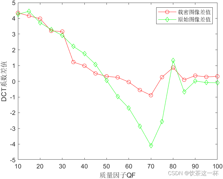 Figure 9
task5: Use 84 images in the standard library for testing, and set the quality factor QF=70. In this case, calculate the difference between the DCT coefficient of the secret image and the reference image. The DCT coefficient of the original compressed image is 0 digits and the DCT coefficient of the reference image is 0 digits. The plot is shown in Figure 10. It can be seen that the difference of the densified image is basically greater than the difference of the original image. It is determined that the difference of the densified image is accurate. According to this alignment, 168 images (84 classified images and 84 non-classified images) were classified into image types, and the classification accuracy was 95.24% (as shown in Figure 11);
 Figure 10

Figure 11
4. Summary discussion and exploration
This experiment analyzes whether JPEG images are steganographic. There are two main methods of analysis: block eigenvalue detection and DCT coefficient histogram anomaly detection. Regarding the two detection methods, I went from the shallower to the deeper in this experiment. From the beginning, I only needed to determine that the block feature value of the image to be tested (the number of DCT coefficients with 0) is greater than the block feature value of the reference image. (The number of DCT coefficients of 0) can be determined to be a dense image. Later, the block feature value of the image to be tested (the number of DCT coefficients of 0) is greater than the block feature value of the reference image (the DCT coefficient of 0). (number), and then use a large number of (84) standard images to determine the defining value of the image type in the later stage, and finally obtain a good judgment result.
However, there are more reasonable methods for steganography detection of JPEG images. Compared with the method of this experiment, the method is divided into finding the limit value and using machine learning methods (of which SVM support vector machine is the most suitable). By detecting a large amount of data, you can determine whether the JPEG image has been steganographically based on the characteristic values of the image.
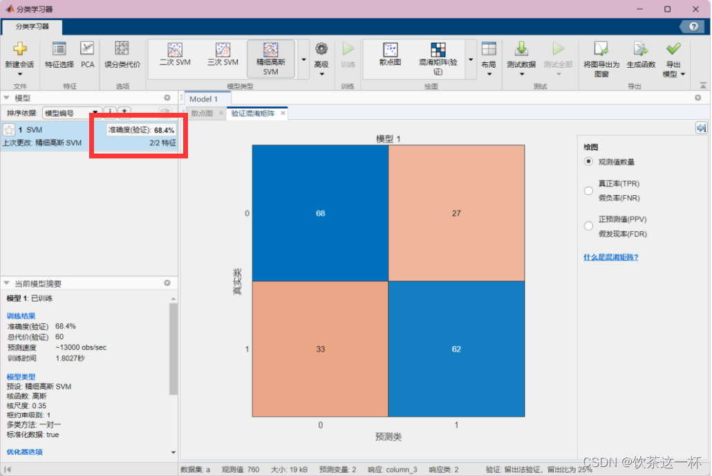
The first time I tried to use matlab to write an SVM program, I found that the program was too complicated. Just when I was about to give up, I found that matlab has its own SVM toolbox. I used matlab's own classification learning tool and used a data set with two dimensions (dimension). Block feature value and image quality factor QF), 760 data are selected for training.
Select Fine Gaussian SVM learning, and the learning results are as follows:

5. Appendix code
task1.m
%% 环境初始化
clc
clear
close all
cover=imread('./test/Lena.bmp');
[h,w]=size(cover);
max_len=(h/8)*(w/8);
ER=max_len/(h*w);       %只能保证每8*8的方块中最少存在一个非零值,最大嵌入率
flag=zeros(numel(10:5:100),1);    %标记每次提取数据与嵌入数据是否一致

%% 读取测试图像
stego=cell(numel(10:5:100),1);      %存储载密矩阵
k1=1;
B_0=zeros(numel(10:5:100),1);        %载体压缩图像的分块特征值
filename='./test/Lena';
B_1=zeros(numel(10:5:100),1);   %载密图像的分块特征值
B_e=zeros(numel(10:5:100),1);   %载密参考图像的分块特征值
B_e_0=zeros(numel(10:5:100),1);   %原始参考图像的分块特征值的
for qf=10:5:100
    ImgName = getJPEG(filename,qf);
    %% 计算压缩图像的分块特征值
    cover=imread(ImgName);
    B_0(k1)=block(cover);
    data_len=floor(ER*(h*w));                       %总嵌入长度为data_len比特
    data_in=round(rand(floor(data_len/3),1)*7);     %随机数为8进制数,即一个数占3bit,总嵌入长度为data_len比特
    %% F5隐写
    stego = F5_in(cover,data_in);
    %% F5提取并将嵌入数据与提取数据进行对比
    data_out=F5_out(stego,ER);
    if isequal(data_in,data_out)
        %disp("F5算法嵌入的数据与提取的数据完全一致");
        flag(k1)=1;
    end
    %% 计算载密图像的分块特征值
    B_1(k1)=block(stego);
    %% 计算参考图像的分块特征值
    stego_e=stego(5:h,:);
    cover_e=cover(:,5:w);
    B_e(k1)=block(stego_e);
    B_e_0(k1)=block(cover_e);
    k1=k1+1;
end
%% 分块特征值分析
figure();
plot(10:5:100,B_0,'r-v',10:5:100,B_e_0,'g-o',10:5:100,B_1,'b-^',10:5:100,B_e,'k-d');
xlabel("质量因子QF");
ylabel("分块特征值");
legend(["原始图像","原始参考图像","载密图像","载密参考图像"]);
%% 检测提取数据是否与嵌入数据完全一致
if isequal(flag,ones(numel(10:5:100),1))
    disp("提取数据与嵌入数据完全一致");
else
    rate=(sum(sum(flag))*1+sum(sum(flag==0))*0.99)/(numel(10:5:100)*numel(0.001:0.001:ER_max));
    disp("嵌入与提取总次数");numel(10:5:100)*numel(0.001:0.001:ER_max)
    disp("出错次数");sum(sum(flag==0))
    disp("数据正确提取比率");rate
end
task2.m
%% 环境初始化
clc
clear
close all
cover=imread('./test/test_more/1.bmp');
[h,w]=size(cover);
max_len=(h/8)*(w/8);
ER=max_len/(h*w);       %只能保证每8*8的方块中最少存在一个非零值,最大嵌入率

%% 读取测试图像
B_1=zeros(numel(10:5:100),20);   %载密图像的分块特征值
B_e=zeros(numel(10:5:100),20);   %参考图像的分块特征值
B_0=zeros(numel(10:5:100),20);   %载体压缩图像的分块特征值
B_0_e=zeros(numel(10:5:100),20);   %载体压缩图像的分块特征值
for num=1:20
    stego=cell(numel(10:5:100),1);          %存储载密矩阵
    k1=1;
    filename=['./test/test_more/',num2str(num)];
    for qf=10:5:100
        ImgName = getJPEG(filename,qf);
        %% 计算压缩图像的分块特征值
        cover=imread(ImgName);
        B_0(k1,num)=block(cover);
        data_len=floor(ER*(h*w));                       %总嵌入长度为data_len比特
        data_in=round(rand(floor(data_len/3),1)*7);     %随机数为8进制数,即一个数占3bit,总嵌入长度为data_len比特
        %% F5隐写
        stego{k1} = F5_in(cover,data_in);
        %% 计算载密图像的分块特征值
        B_1(k1,num)=block(stego{k1});
        %% 计算参考图像的分块特征值
        stego_e=stego{k1}(:,5:w);
        cover_e=cover(:,5:w);
        B_0_e(k1,num)=block(stego_e);
        B_e(k1,num)=block(stego_e);
        k1=k1+1;
    end
end
%% 分块特征值分析
figure();
B_0_dif=B_0-B_0_e;
B_1_dif=B_1-B_e;
B_diff=B_1_dif-B_0_dif;
line=zeros(19,20);
surf(1:20,1:19,B_diff);
hold on;
surf(1:20,1:19,line);
xlabel("图像序号");
ylabel("质量因子QF");
zlabel("分块特征值差值");
%% 确定差值准线
m1=mean(B_1_dif,"all");
m0=mean(B_0_dif,"all");
figure();
plot(1:20,ones(1,20)*m0,'r-',1:20,ones(1,20)*m1,'b-');
for k=1:19
    hold on;
    plot(1:20,B_0_dif(k,:),'r+');
    plot(1:20,B_1_dif(k,:),'b+');
end
legend("原始图像差值均值","载密图像差值均值","原始图像差值","载密图像差值");
task3.m
%% 环境初始化
clc
clear
close all
cover=imread('./test/test_more/1.bmp');
[h,w]=size(cover);
max_len=(h/8)*(w/8);
ER=max_len/(h*w);       %只能保证每8*8的方块中最少存在一个非零值,最大嵌入率

%% 读取测试图像
B_1=zeros(1,84);   %载密图像的分块特征值
B_e=zeros(1,84);   %参考图像的分块特征值
B_0=zeros(1,84);   %载体压缩图像的分块特征值
B_0_e=zeros(1,84);   %载体压缩图像的分块特征值
for num=1:84
    k1=1;
    filename=['./test/test_more/',num2str(num)];
    qf=70;
    ImgName = getJPEG(filename,qf);
    %% 计算压缩图像的分块特征值
    cover=imread(ImgName);
    B_0(k1,num)=block(cover);
    data_len=floor(ER*(h*w));                       %总嵌入长度为data_len比特
    data_in=round(rand(floor(data_len/3),1)*7);     %随机数为8进制数,即一个数占3bit,总嵌入长度为data_len比特
    %% F5隐写
    stego = F5_in(cover,data_in);
    %% 计算载密图像的分块特征值
    B_1(k1,num)=block(stego);
    %% 计算参考图像的分块特征值
    stego_e=stego(:,5:w);
    cover_e=cover(:,5:w);
    B_0_e(k1,num)=block(stego_e);
    B_e(k1,num)=block(stego_e);
    k1=k1+1;
end
%% 分块特征值分析
figure();
B_0_dif=B_0-B_0_e;
B_1_dif=B_1-B_e;
plot(1:84,max(B_0_dif)*ones(84,1),'r-',1:84,B_0_dif,'r-d',1:84,B_1_dif,'g-o');
xlabel("图像序号");
zlabel("分块特征值差值");
legend("原始图像差值准线","原始图像差值","载密图像差值");
%% JPEG结果分析判断
flag=zeros(84*2);       %标记图像是否为隐写图像
for k2=1:84
    if B_1_dif(k2)>=max(B_0_dif)    %差值足够大,判定为隐写图像
        flag(k2)=1;
    else                    %差值不足够大,判定为非隐写图像
        flag(k2)=0;
    end
    if B_0_dif(k2)<max(B_0_dif)
        flag(84+k2)=0;
    else
        flag(84+k2)=1;
    end
end
right_rate=(sum(sum(flag(1:84,:)==1))+sum(sum(flag(85:84*2,:)==0)))/(84*2);
disp("检测正确率为");right_rate
task4.m
%% 环境初始化
clc
clear
close all
cover=imread('./test/Lena.bmp');
[h,w]=size(cover);
max_len=(h/8)*(w/8);
ER=max_len/(h*w);       %只能保证每8*8的方块中最少存在一个非零值,最大嵌入率

%% 读取测试图像
stego=cell(numel(10:5:100),1);          %存储载密矩阵
k1=1;
filename='./test/Lena';
y_dif1=zeros(19,1);
y_dif0=zeros(19,1);
for qf=10:5:100
    ImgName = getJPEG(filename,qf);
    %% 计算压缩图像的直方图
    cover=imread(ImgName);
    y0=statistics(cover);
    data_len=floor(ER*(h*w));                       %总嵌入长度为data_len比特
    data_in=round(rand(floor(data_len/3),1)*7);     %随机数为8进制数,即一个数占3bit,总嵌入长度为data_len比特
    %% F5隐写
    stego{k1} = F5_in(cover,data_in);
    %% 计算载密图像的直方图
    y1=statistics(stego{k1});
    %% 计算参考图像的直方图
    stego_e=stego{k1}(:,5:w);
    cover_e=cover(:,5:w);
    y2=statistics(stego_e);
    y3=statistics(cover_e);
    p1=find(y1(:,1)==0);
    p2=find(y2(:,1)==0);
    p0=find(y0(:,1)==0);
    p3=find(y3(:,1)==0);
    figure();
    plot(y0(p0-5:p0+5,1),y0(p0-5:p0+5,2),'r-o',y3(p3-5:p3+5,1),y3(p3-5:p3+5,2),'k-v',y1(p1-5:p1+5,1),y1(p1-5:p1+5,2),'b-^',y2(p2-5:p2+5,1),y2(p2-5:p2+5,2),'g-d');
    legend(["原始图像","原始参考图像","载密图像","载密参考图像"]);
    %% 数据处理
    y_dif1(k1)=y1(p1,3)-y2(p2,3);
    y_dif0(k1)=y0(p0,3)-y3(p3,3);
    k1=k1+1;
end
%% 数据分析
figure();
plot(10:5:100,y_dif1,'r-o',10:5:100,y_dif0,'g-d');
legend("载密图像差值","原始图像差值");
xlabel("质量因子QF");
ylabel("DCT系数差值");
task5.m
%% 环境初始化
clc
clear
close all
cover=imread('./test/test_more/1.bmp');
[h,w]=size(cover);
max_len=(h/8)*(w/8);
ER=max_len/(h*w);       %只能保证每8*8的方块中最少存在一个非零值,最大嵌入率

%% 读取测试图像
y_dif1=zeros(84,1);
y_dif0=zeros(84,1);
k1=1;
for num=1:84
    %stego=cell(numel(10:5:100),1);          %存储载密矩阵
    filename=['./test/test_more/',num2str(num)];
    qf=70;
    ImgName = getJPEG(filename,qf);
    %% 计算压缩图像的直方图
    cover=imread(ImgName);
    y0=statistics(cover);
    data_len=floor(ER*(h*w));                       %总嵌入长度为data_len比特
    data_in=round(rand(floor(data_len/3),1)*7);     %随机数为8进制数,即一个数占3bit,总嵌入长度为data_len比特
    %% F5隐写
    stego = F5_in(cover,data_in);
    %% 计算载密图像的直方图
    y1=statistics(stego);
    %% 计算参考图像的直方图
    stego_e=stego(:,5:w);
    y2=statistics(stego_e);
    cover_e=cover(:,5:w);
    y3=statistics(cover_e);
    p1=find(y1(:,1)==0);
    p2=find(y2(:,1)==0);
    p0=find(y0(:,1)==0);
    p3=find(y3(:,1)==0);
    %% 数据处理
    y_dif1(k1)=y1(p1,3)-y2(p2,3);
    y_dif0(k1)=y0(p0,3)-y3(p3,3);
    k1=k1+1;
end
%% 数据分析
figure();
plot(1:84,y_dif1,'r-d',1:84,y_dif0,'g-o',1:84,min(y_dif1)*ones(84,1),'r-');
xlabel("图像编号");
ylabel("DCT系数差值");
legend("载密图像差值","原始图像差值","载密图像差值准线");
%% JPEG结果分析判断
flag=ones(84*2,1)*2;       %标记图像是否为隐写图像
for k1=1:84
    if y_dif1(k1)>=min(y_dif1)
        flag(k1)=1;
    else
        flag(k1)=0;
    end
    if y_dif0(k1)<=min(y_dif1)
        flag(84+k1)=0;
    else
        flag(84+k1)=1;
    end
end
right_rate=(sum(sum(flag(1:84)==1))+sum(sum(flag(85:168)==0)))/(84*2);
disp("检测正确率为");right_rate
This article is original and may not be reproduced without the consent of the author! ! !
Complete code (can be run directly) steganalysis (including all codes and test data)-Matlab document resources-CSDN library ![]() https://download.csdn.net/download/HUANGliang_/86262110
https://download.csdn.net/download/HUANGliang_/86262110