PyTorch study notes 2: nn.Module, optimizer, model saving and loading, TensorBoard

Reference: "Summary of PyTorch study notes (completed with flowers)" , PyTorch Chinese official tutorial , PyTorch official website

1. nn.Module

1.1 Call of nn.Module

Pytorch implements the construction of deep learning models by inheriting the nn.Module class and defining the instantiation and forward propagation of sub-modules. Its construction code is as follows:

import torch
import torch.nn as nn

class Model(nn.Module):
    def __init__(self, *kargs): # 定义类的初始化函数，...是用户的传入参数
        super(Model, self).__init__()#调用父类nn.Module的初始化方法
        ... # 根据传入的参数来定义子模块
    
    def forward(self, *kargs): # 定义前向计算的输入参数，...一般是张量或者其他的参数
        ret = ... # 根据传入的张量和子模块计算返回张量
        return ret

• The __init__ method initializes the entire model
• super(Model, self).__init__(): Call the initialization method of the parent class nn.Module to initialize the necessary variables and parameters
• Define forward propagation module

1.2 Implementation of linear regression

import torch
import torch.nn as nn

class LinearModel(nn.Module):
    def __init__(self, ndim):
        super(LinearModel, self).__init__()
        self.ndim = ndim#输入的特征数

        self.weight = nn.Parameter(torch.randn(ndim, 1)) # 定义权重
        self.bias = nn.Parameter(torch.randn(1)) # 定义偏置

    def forward(self, x):
        # 定义线性模型 y = Wx + b
        return x.mm(self.weight) + self.bias

• Define weights and biases self.weight and self.bias. Initialize using standard normal distribution torch.randn.
• self.weight and self.bias are parameters of the model, which are wrapped using nn.Parameter to convert these initialized tensors into parameters of the model. Only parameters can be optimized (accessed by the optimizer)

The instantiation method is as follows:

lm = LinearModel(5) # 定义线性回归模型，特征数为5
x = torch.randn(4, 5) # 定义随机输入，迷你批次大小为4
lm(x) # 得到每个迷你批次的输出

1. Use model.named_parameters() or model.parameters() to get the generator of model parameters. The difference is that the former contains parameter names and corresponding tensor values, while the latter only contains tensor values.
2. The optimizer optimzer directly accepts the parameter generator as a parameter, and optimizes all tensors in the generator according to the gradient during backpropagation.
3. The role of model.train() is to enable Batch Normalization and Dropout. The function of model.eval() is to disable Batch Normalization and Dropout.
4. named_buffers and buffers get the cache of tensors (parameters that do not participate in gradient propagation but will be updated, such as the mean and variance of BN) register_buffers can join this tensor
5. Use apply to recursively apply functions to submodules (can be anonymous function lambda)

For further information on the usage and differences between model.train() and model.eval(), please refer to: "Pytorch: Usage and Differences between model.train() and model.eval()"

For example, take the linear model defined above:

lm.named_parameters() # 获取模型参数（带名字）的生成器
#<generator object Module.named_parameters at 0x00000279A1809510>
list(lm.named_parameters()) # 转换生成器为列表

[('weight',
  Parameter containing:
  tensor([[-1.0407],
          [ 0.0427],
          [ 0.4069],
          [-0.7064],
          [-1.1938]], requires_grad=True)),
 ('bias',
  Parameter containing:
  tensor([-0.7493], requires_grad=True))]
  
lm.parameters() # 获取模型参数（不带名字）的生成器
list(lm.parameters()) # 转换生成器为列表

[Parameter containing:
 tensor([[-1.0407],
         [ 0.0427],
         [ 0.4069],
         [-0.7064],
         [-1.1938]], requires_grad=True),
 Parameter containing:
 tensor([-0.7493], requires_grad=True)]

lm.cuda()#模型参数转到GPU上
list(lm.parameters()) # 转换生成器为列表

• model.train() ensures that the BN layer can use the mean and variance of each batch of data. For Dropout, model.train() randomly removes neurons during training and uses part of the network connections to train and update parameters. If the deleted neuron (cross) is the only neuron contributing to the correct result. Once we remove the deleted neuron, it forces other neurons to train and learn how to remain accurate without the deleted neuron. This dropout improves the performance in the final test, but it negatively affects the performance during training because the network is incomplete

• Add model.eval() when testing. model.eval() ensures that the BN layer can use the mean and variance of all training data, that is, the mean and variance of the BN layer must remain unchanged during the test process (when model.eval(), the framework will automatically fix the BN and Dropout , will not average, directly use the mean and var values ​​that have been learned in the training stage)

2. Loss function

Refer to "Summary of Commonly Used Loss Functions in Machine Learning"

The pytorch loss function comes in two forms:

• The function form called by torch.nn.functional . Pass in the neural network prediction value and target value to calculate the loss function
• Module form in the torch.nn library . Create an instance of the module and call the modular method to calculate
  . The final output is a scalar. There are two reduction methods for the value of the loss function of a batch: summation and averaging.

1. Regression problems generally call the torch.nn.MSEloss module. Create an instance using default parameters, and the output is the mean value of the loss function for a batch.

import torch
import torch.nn as nn
mse = nn.MSELoss() # 初始化平方损失函数模块
#class torch.nn.MSELoss(size_average=None, reduce=None, reduction='mean')
t1 = torch.randn(5, requires_grad=True) # 随机生成张量t1
tensor([ 0.6582,  0.0529, -0.9693, -0.9313, -0.7288], requires_grad=True)

t2 = torch.randn(5, requires_grad=True) # 随机生成张量t2
tensor([ 0.8095, -0.3384, -0.9510,  0.1581, -0.1863], requires_grad=True)

mse(t1, t2) # 计算张量t1和t2之间的平方损失函数
tensor(0.3315, grad_fn=<MseLossBackward>)

2. Two classification problem:
   • Use torch.nn.BCELoss binary cross-entropy loss function. The output is the mean value of the loss function. Accepts two tensors. The former is the probability value of the positive classification label (the predicted value must be outputted through nn.Sigmoid() probability), and the latter is the target data value of the two-class label (1 is positive classification). Both must be of floating point type.
   • torch.nn.BCEWithLogitsLoss : Automatically implements the function of the sigmoid function inside the loss function, which can increase the stability of the calculation. Because when the probability is close to 0 or 1, the logarithmic part accepted by the binary cross-entropy loss function is easy to approach infinity, causing numerical instability. Use torch.nn.BCEWithLogitsLoss to avoid this situation

t1s = torch.sigmoid(t1)
t2 = torch.randint(0, 2, (5, )).float() # 随机生成0，1的整数序列，并转换为浮点数
bce=torch.nn.BCELoss()
(t1s, t2) # 计算二分类的交叉熵
bce_logits = nn.BCEWithLogitsLoss() # 使用交叉熵对数损失函数
bce_logits(t1, t2) # 计算二分类的交叉熵，可以发现和前面的结果一致

3. Multi-classification problem
   • torch.nn.NLLLoss : Negative logarithmic loss function. Before calculation, the predicted value must go through the softmax function to output the probability value ( torch.nn.functional.log_softmax or torch.nn.LogSoftmax(dim=dim) function )
   • torch.nn.CrossEntropyLoss : Cross entropy loss function, the softmax output probability has been integrated internally, and there is no need to perform softmax calculation on the predicted value.

N=10 # 定义分类数目
t1 = torch.randn(5, N, requires_grad=True) # 随机产生预测张量
t2 = torch.randint(0, N, (5, )) # 随机产生目标张量
t1s = torch.nn.functional.log_softmax(t1, -1) # 计算预测张量的LogSoftmax
nll = nn.NLLLoss() # 定义NLL损失函数
nll(t1s, t2) # 计算损失函数
ce = nn.CrossEntropyLoss() # 定义交叉熵损失函数
ce(t1, t2) # 计算损失函数，可以发现和NLL损失函数的结果一致

3. Optimizer

For more learning rate optimizers and schedulers, please refer to "torch.optim Official Documentation"

3.1.1 SGD optimizer

Taking the Boston housing price problem as an example, we build an SGD optimizer. The first parameter is the model's parameter generator (called by lm.parameters()), and the second parameter is the learning rate. Optimization calculations are performed through optim.step() during training.

from sklearn.datasets import load_boston
boston = load_boston()

lm = LinearModel(13)
criterion = nn.MSELoss()
optim = torch.optim.SGD(lm.parameters(), lr=1e-6) # 定义优化器
data = torch.tensor(boston["data"], requires_grad=True, dtype=torch.float32)
target = torch.tensor(boston["target"], dtype=torch.float32)

for step in range(10000):
    predict = lm(data) # 输出模型预测结果
    loss = criterion(predict, target) # 输出损失函数
    if step and step % 1000 == 0 :
        print("Loss: {:.3f}".format(loss.item()))
    optim.zero_grad() # 清零梯度
    loss.backward() # 反向传播
    optim.step()

torch.optim.SGD(params,lr=<required parameter>,momentum=0,
    dampening=0,weight_decay=0,nesterov=False)

#momentum：动量因子
#dampening：动量抑制因子
#nesterov：设为True时使用nesterov动量

3.1.2 Adagrad optimizer

torch.optim.Adagrad(
    params,lr=0.01,lr_decay=0,weight_decay=0,
    initial_accumulator_value=0,eps=1e-10)

#lr_decay：学习率衰减速率
#weight_decay：权重衰减
#initial_accumulator_value：梯度初始累加值

3.2 Hierarchical learning rate

Specify different learning rates for different parameters:

optim.SGD([
                {
    
    'params': model.base.parameters()},
                {
    
    'params': model.classifier.parameters(), 'lr': 1e-3}
            ], lr=1e-2, momentum=0.9)

This means that the parameters of model.base will use the default learning rate of 1e-2, the parameters of model.classifier will use the learning rate of 1e-3, and all parameters of 0.9 will use momentum.

3.3 Learning rate scheduler torch.optim.lr_scheduler

For more learning rate optimizers and schedulers, please refer to "torch.optim Official Documentation"

scheduler = StepLR(optimizer, step_size=30, gamma=0.1)
#没经过30的个迭代周期，学习率降为原来的0.1倍。每个epoch之后学习率都会衰减。
or epoch in range(100):
    train(...)
    validate(...)
    scheduler.step()

Most learning rate schedulers can be called back-to-back (also called chain schedulers). The result is that each scheduler is applied one after the other to the learning rate obtained by the previous scheduler.

example:

model = [Parameter(torch.randn(2, 2, requires_grad=True))]
optimizer = SGD(model, 0.1)
scheduler1 = ExponentialLR(optimizer, gamma=0.9)
scheduler2 = MultiStepLR(optimizer, milestones=[30,80], gamma=0.1)

for epoch in range(20):
    for input, target in dataset:
        optimizer.zero_grad()
        output = model(input)
        loss = loss_fn(output, target)
        loss.backward()
        optimizer.step()
    scheduler1.step()
    scheduler2.step()

4. Data loading torch.utils.data

You can also refer to this section "Writing a custom pytorch training loop for transformers (Dataset and DataLoader analysis and example code)"

4.1 DataLoader parameters

The core of PyTorch's data loading utilities is the torch.utils.data.DataLoader class. It represents a Python iterable data set, supporting:

• map type and iterable type data sets
• Custom data loading order
• Automatic batching
• Single-process and multi-process data loading

train_loader = DataLoader(dataset=train_data, batch_size=6, shuffle=True ，num_workers=4)
test_loader = DataLoader(dataset=test_data, batch_size=6, shuffle=False，num_workers=4)

Let’s take a look at the dataloader code:

class DataLoader(object):
    def __init__(self, dataset, batch_size=1, shuffle=False, sampler=None,
                 batch_sampler=None, num_workers=0, collate_fn=None,
                 pin_memory=False, drop_last=False, timeout=0,
                 worker_init_fn=None,*, prefetch_factor=2,persistent_workers=False)
    self.dataset = dataset
        self.batch_size = batch_size
        self.num_workers = num_workers
        self.collate_fn = collate_fn
        self.pin_memory = pin_memory
        self.drop_last = drop_last
        self.timeout = timeout
        self.worker_init_fn = worker_init_fn

• dataset:Dataset class, PyTorch’s existing data reading interface, determines where and how to read data;
• batch_size: batch size; default 1
• num_works: Whether to use multiple processes to read data; the default is 0 to use the main process to import data. If it is greater than 0, multiple processes will import data to speed up data import.
• shuffle: Whether each epoch is shuffled; default False. The order of input data is scrambled to make the data more independent. However, if the data has sequence characteristics, do not set it to True. Generally, shuffling the training set is sufficient.
• drop_last: When the number of samples cannot be divided by batchsize, whether to discard the last batch of data;
• collate_fn: Collate the obtained data into a batch. The default setting is False. If set to True, the system will copy tensor data (Tensors) to CUDA memory before returning.
• batch_sampler, batch sampling, and batch_size, shuffle and other parameters are mutually exclusive, and the default None is generally used. batch_sampler, but each time it returns the index of a batch of data (note: not data), the data input to the network should be in a random sampling mode each time, which can make the data more independent. Therefore, it is incompatible with the sequential input of bundles, data shuffling, data sampling, etc. modes.
• sampler, default False. Sampling inputs from a data set according to a defined strategy. If a sampling rule is defined, the shuffle setting must be False.
• pin_memory, memory storage, default is False. Whether to copy data to CUDA memory before data is returned.
• timeout is used to set the timeout for data reading, but if the data is not read beyond this time, an error will be reported.
• worker_init_fn (data type callable), subprocess import mode, default is Noun. Before the data is imported and after the step is completed, the data is imported in order one by one according to the ID of the working sub-process.

If you want to load the input with randomly selected patterns, you can set sampler or batch_sampler. How to define sampling rules, you can read the sampler.py script, or this post: "Understand the relationship between Pytorch's DataLoader, DataSet, and Sampler in one article"

4.2 Two data set types

The most important parameter of the DataLoader constructor is dataset, which represents the dataset object from which data is to be loaded. PyTorch supports two different types of datasets:

• map-style datasets: mapping type datasets. Each data has a corresponding index. By entering the specific index, you can get the corresponding data.

Its construction method is as follows:

class Dataset(object):
    def __getitem__(self, index):
        # index: 数据缩索引（整数，范围为0到数据数目-1）
        # ...
        # 返回数据张量

    def __len__(self):
        # 返回数据的数目
        # ...

Mainly rewrite two methods:

• __getitem__: Python's built-in operator method, corresponding to the index operator []. By inputting an integer index, a specific piece of data is returned. The specific internal logic depends on the data set type.
• __len__: Returns the total number of data

For more details, please refer to "torch.utils.data.Dataset"

• iterable-style datasets: Iterable datasets: instances of subclasses that implement the __iter__() protocol. No need for __getitem__ and __len__ methods, it is actually similar to python's iterator
• Unlike mappings, indexes are independent of each other. When multi-threaded loading occurs, multiple threads allocate indexes independently. When indexing the right context during iteration, you need to consider how to split the data.
• This type of data set is particularly useful in situations where random reads are expensive or even impossible, and where the batch size depends on the data being acquired.
• When calling iter(dataset), you can return a data stream read from a database, a remote server, or even a log generated in real time.

class MyIterableDataset(torch.utils.data.IterableDataset):
    def __init__(self, start, end):
        super(MyIterableDataset).__init__()
            assert end > start, \
"this example code only works with end >= start"
            self.start = start
            self.end = end

    def __iter__(self):
        worker_info = torch.utils.data.get_worker_info()
        if worker_info is None:  # 单进程数据载入
            iter_start = self.start
            iter_end = self.end
        else:  # 多进程，分割数据
        	   #根据不同工作进程序号worker_id，设置不同进程数据迭代器取值范围。保证不同进程获取不同的迭代器。
            per_worker = int(math.ceil((self.end - self.start) \
                            / float(worker_info.num_workers)))
            worker_id = worker_info.id
            iter_start = self.start + worker_id * per_worker
            iter_end = min(iter_start + per_worker, self.end)
        return iter(range(iter_start, iter_end))

See IterableDataset for more details

4.3 Data loading sequence and Sampler

• For iterable-style datasets, the data loading order is completely controlled by the user-defined iterable. This allows for easier implementation of block reads and dynamic batch sizes (e.g., by producing a batch of samples each time).
• For map type data, the torch.utils.data.Sampler class is used to specify the sequence of indexes/keys used in data loading. They represent iterable objects over the dataset index. For example, in the common case of stochastic gradient descent (SGD), Sampler can shuffle the index list and produce one at a time, or produce a small number of indices for mini-batch SGD.

A sequential or shuffled sampler DataLoader will be automatically built based on shufflea's parameters. Alternatively, the user can use the sampler parameter to specify a custom Sampler object that generates the next index/key to fetch each time.

Customization of the batch index list generated once by the Sampler can be passed as the batch_sampler parameter. Automatic batching can also be enabled via the batch_size and drop_last parameters.

4.4 Batch processing and collate_fn

DataLoader supports batching data via the parameters batch_size, drop_last and batch_sampler.
When automatic batching is enabled, collate_fn is called each time with a list of data samples. Expected to collate input samples into a batch to be produced from the data loader iterator.

For example, if each data sample consists of a 3-channel image and a complete class label, i.e. a tuple (image, class_index) is returned for each element of the dataset, then the default collate_fn will be a list of such tuples Arrange into a single tuple a batched image tensor and a batched class labels tensor. In particular, the default collate_fn has the following properties:

• It always prepends a new dimension as the batch dimension.

• It automatically converts NumPy arrays and Python numbers into PyTorch tensors.

• It preserves the data structure, e.g. if each sample is a dictionary, it outputs a dictionary with the same set of keys but batches of tensors as values ​​(or lists if the values ​​cannot be converted to tensors). The same goes for list s, tuples, namedtuple s, etc.

Users can use a custom collate_fn to implement custom batching, for example, collate along dimensions other than the first, fill sequences of various lengths, or add support for custom data types.

5. Saving and loading models

5.1 Serialization and deserialization of modules and tensors

• PyTorch modules and tensors are essentially instances of the torch.nn.Module and torch.tensor classes. PyTorch comes with a series of methods that can convert instances of these classes into strings of words . So these instances can be serialized and deserialized via Python serialization methods.
• Tensor serialization: Essentially, the tensor information, including data type and storage location, as well as the data carried, is converted into a string, and then stored using Python's own file IO function . Of course, this process is reversible.

torch.save(obj, f, pickle_module=pickle, pickle_protocol=2)
torch.load(f, map_location=None, pickle_module=pickle, **pickle_load_args)

• torch.save parameter

  1. Objects that can be serialized in pytorch, including models and tensors
  2. Storage file path
  3. Serialization library, pickle by default
  4. pickle protocol, versions 0-4

• torch.load function

  1. file path
  2. Mapping of tensor storage locations (default CPU, can also be GPU)
  3. The pickle parameter is the same as when saving.

  If the model is saved in the GPU and the current computer being loaded does not have a GPU, or the GPU device number is incorrect, you can use map_location='cpu'.

PyTorch has two model saving methods by default:

• Save an instance of the model
• Save the model's state dictionary state_dict: state_dict contains all parameter names and corresponding tensors of the model. By calling load_state_dict, you can obtain the state dictionary of the current model and load the model parameters.

5.2 state_dict saves model parameters

torch.save(model.state_dict(), PATH)
model = TheModelClass(*args, **kwargs)
model.load_state_dict(torch.load(PATH))
model.eval()

• Save the model state dictionary state_dict: only saves the parameters learned by the model, which is less related to the module, that is, it does not depend on the version.
• The most common model saving in PyTorch uses '.pt' or '.pth' as ​​the model file extension.
• Before running inference, be sure to call model.eval() to set the dropout and batch normalization layers to evaluation
  mode. Failure to do so may result in inconsistent model inference results.

5.2 Save/load complete model

Save the model using the Python `pickle module. The disadvantages of this approach are:

• Serialized data is restricted to a special class and requires an exact dictionary structure. When used in other projects or refactored, your code may break in various ways.
• The implementation of PyTorch modules depends on the specific version. Module serialization files saved in one version may not be loaded in another version.

torch.save(model, PATH)
# 模型类必须在此之前被定义
model = torch.load(PATH)
model.eval()

5.3 Checkpoint is used for inference/continuation of training

• During training, not only model-related information must be saved, but also optimizer-related information must be saved. Because it may be necessary to start from the checkpoint and continue training. Therefore, the state dictionary of the optimizer itself can be saved, storing information including the current learning rate, scheduler, etc.
• The latest recorded training losses, external torch.nn.Embedding layers, etc. can be saved.
• A common way to save checkpoints in PyTorch is to use the .tar file extension.
• To load the project, you first need to initialize the model and optimizer, then use torch.load() to load the local dictionary

The checkpoint code for a model is as follows:

torch.save({
    
    
'epoch': epoch,
'model_state_dict': model.state_dict(),
'optimizer_state_dict': optimizer.state_dict(),
'loss': loss,
...
}, PATH)

load

model = TheModelClass(*args, **kwargs)
optimizer = TheOptimizerClass(*args, **kwargs)
checkpoint = torch.load(PATH)
model.load_state_dict(checkpoint['model_state_dict'])
optimizer.load_state_dict(checkpoint['optimizer_state_dict'])
epoch = checkpoint['epoch']
loss = checkpoint['loss']
model.eval()#或model.train()

or it could be:

save_info = {
    
     # 保存的信息
    "iter_num": iter_num,  # 迭代步数 
    "optimizer": optimizer.state_dict(), # 优化器的状态字典
    "model": model.state_dict(), # 模型的状态字典
}
# 保存信息
torch.save(save_info, save_path)
# 载入信息
save_info = torch.load(save_path)
optimizer.load_state_dict(save_info["optimizer"])
model.load_state_dict(sae_info["model"])

5.4 Saving multiple models in one file

torch.save({
    
    
'modelA_state_dict': modelA.state_dict(),
'modelB_state_dict': modelB.state_dict(),
'optimizerA_state_dict': optimizerA.state_dict(),
'optimizerB_state_dict': optimizerB.state_dict(),
...
}, PATH)

load

modelA = TheModelAClass(*args, **kwargs)
modelB = TheModelBClass(*args, **kwargs)
optimizerA = TheOptimizerAClass(*args, **kwargs)
optimizerB = TheOptimizerBClass(*args, **kwargs)
checkpoint = torch.load(PATH)
modelA.load_state_dict(checkpoint['modelA_state_dict'])
modelB.load_state_dict(checkpoint['modelB_state_dict'])
optimizerA.load_state_dict(checkpoint['optimizerA_state_dict'])
optimizerB.load_state_dict(checkpoint['optimizerB_state_dict'])
modelA.eval()
modelB.eval()

  When saving a model composed of multiple torch.nn.Modules, such as GAN (generative adversarial network), sequence-to-sequence (sequence-to-sequence model), or fusion of multiple models, the same method as saving regular checkpoints can be used Methods. In other words, save a dictionary of each model's state_dict and the corresponding optimizer. As mentioned before, any additional items can be saved by simply appending them to the dictionary, which will aid in resuming training.

6. Installation and use of TensorBoard

Refer to "PyTorch Study Notes (9) ---- Using TensorBoard to Visualize Models, Data and Training"

TensorBoard installation:

pip install tensorflow-tensorboard
pip install tensorboard

  After installation, import tensorboard reported an error: ImportError: TensorBoard logging requires TensorBoard version 1.15 or above. I tried several methods. Finally, close the ipynb file, create a new ipynb file, copy the code and run it.

6.1 Detailed explanation of TensorBoard

TensorBoard is divided into front-end display and back-end data recording, so its Pipeline is also divided into two steps:

Backend data recording : TensorBoard abstracts the backend server into a class: SummaryWriter. After the declaration, the back-end data recording service will be started.

1. Instantiate SummaryWriter

#从tensorboard构造一个摘要写入器SummaryWriter。
from torch.utils.tensorboard import SummaryWriter
writer = SummaryWriter()

The parameters are parsed as follows:

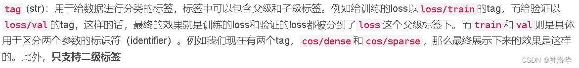
• class SummaryWriter(log_dir=None, comment='', purge_step=None, max_queue=10, flush_secs=120, filename_suffix='')
• log_dir (str): Specifies the location of the folder where the data is saved. If it does not exist, create it.
  • When not specified, the default saved folder is ./runs/current time_host name, for example: Feb04_22-42-47_Alienware.
  • A new folder will be created after each run. Sometimes the model is adjusted from different perspectives, so it is best not to use the default log folder, but to use a meaningful secondary structure, such as: runs/exp1.
• comment (string): The suffix added to the default log_dir. If we have specified the specific value of log_dir, then this parameter will not have any effect.
• purge_step (int)：
  • Visualized data is not written in real time, but in a queue. When the accumulated data exceeds the queue limit, data file writing is triggered. If the written visualization data crashes, the data after purge_step will be discarded.
  • For example, in a certain epoch, when the T + X, that is, the data within the step specified by purge_step are discarded.
• max_queue (int): When recording data, the length of the queue opened in the memory. When the queue is full, the data will be written to the disk (file).
• flush_secs (int): Indicates the time interval (s) for writing tensorboard files. The default is 120 seconds, which is two minutes.
• filename_suffix (string): The suffix added to each file in log_dir, empty by default. For more file name settings, please refer to the tensorboard.summary.writer.event_file_writer.EventFileWriter class.

2. adding data. Instantiate the SummaryWriter class and use the instantiation method to add data. These methods all start with add_, such as: add_scalar, add_scalars, add_image... Specifically, all methods are:

   • add_scalar , add_scalars: add scalar data, such as loss, acc, etc.
   • add_histogram: Add histogram
   • add_graph(): Create Graphs, which store the network structure
   • Other methods
     These methods have common parameters:
     
     

3. View data on the front end

   • tensorboard-logdir./run: Start tensorboard server. The default port is 6006. Visit http://127.0.0.1:6006 to see the tensorboard web interface.
   • writer.close()Services can be turned off

6.2 TensorBoard usage examples

You can also refer to the yolov5 tutorial , which covers the use of tensorboard and clearML.

from sklearn.datasets import load_boston
from torch.utils.tensorboard import SummaryWriter
import torch
import torch.nn as nn

#定义线性回归模型
class LinearModel(nn.Module):
    def __init__(self, ndim):
        super(LinearModel, self).__init__()
        self.ndim = ndim

        self.weight = nn.Parameter(torch.randn(ndim, 1)) # 定义权重
        self.bias = nn.Parameter(torch.randn(1)) # 定义偏置

    def forward(self, x):
        # 定义线性模型 y = Wx + b
        return x.mm(self.weight) + self.bias

boston = load_boston()
lm = LinearModel(13)
criterion = nn.MSELoss()
optim = torch.optim.SGD(lm.parameters(), lr=1e-6)

data = torch.tensor(boston["data"], requires_grad=True, dtype=torch.float32)
target = torch.tensor(boston["target"], dtype=torch.float32)
writer = SummaryWriter() # 构造摘要生成器，定义TensorBoard输出类

for step in range(10000):
    predict = lm(data)
    loss = criterion(predict, target)
    writer.add_scalar("Loss/train", loss, step) # 输出损失函数
    writer.add_histogram("Param/weight", lm.weight, step) # 输出权重直方图
    writer.add_histogram("Param/bias", lm.bias, step) # 输出偏置直方图
    if step and step % 1000 == 0 :
        print("Loss: {:.3f}".format(loss.item()))
    optim.zero_grad()
    loss.backward()
    optim.step()    

Load tensorboard on colab:

%load_ext tensorboard
%tensorboard --logdir runs/swin_s

It can also be called from the command line:

# 打开cmd命令
tensorboard --logdir=.\Chapter2\runs --bind_all
#TensorBoard 2.2.2 at http://DESKTOP-OHLNREI:6006/ (Press CTRL+C to quit)

6.3 Common APIs

SummaryWriter's APIs for adding data all start with add_, specifically:

• 标量类：add_scalar、add_scalars、add_custom_scalars、add_custom_scalars_marginchart、add_custom_scalars_multilinechart、
• Data display class:
  • 图像：add_image、add_images、add_image_with_boxes、add_figure
  • Video: add_video
  • Audio: add_audio
  • Text: add_text
  • Embedding：add_embedding
  • Point cloud: add_mesh
• 统计图：add_histogram、add_histogram_raw、add_pr_curve、add_pr_curve_raw
• Network graph: add_onnx_graph, add_graph
• Hyperparameter map: add_hparams

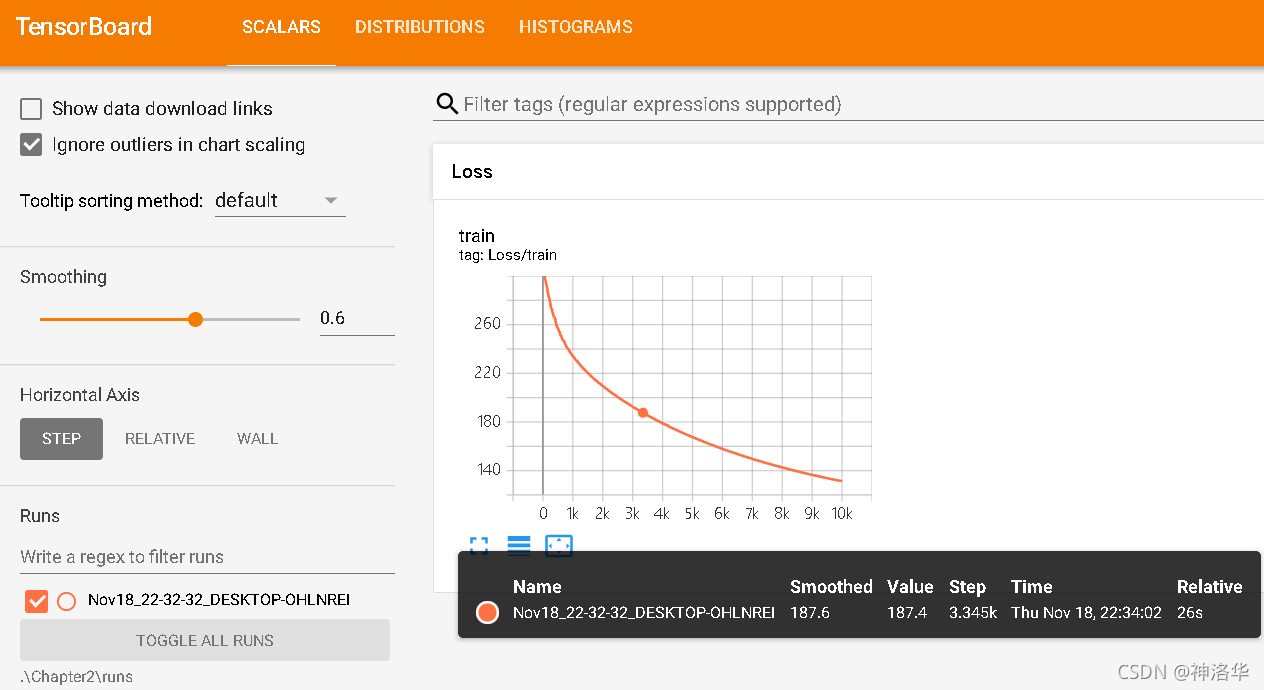
6.3.1 add_scalar() and add_scalars() write scalars

• add_scalar()

add_scalar(tag, scalar_value, global_step=None, walltime=None)

To add loss to tensorboard, common parameters include:
- tag: tags for different charts, such as Train_loss as shown in the figure below.
- scalar_value: the value of the label, a floating point number
- global_step: the current iteration step number, the x-axis coordinate of the label
- walltime: the iteration time function. If not passed in, time.time() is used internally in the method to return a floating point number representing the time.

writer.add_scalar('Train_loss', loss, (epoch*epoch_size + iteration))

• add_scalars()

add_scalars(main_tag, tag_scalar_dict, global_step=None, walltime=None)

Similar to the previous method, each scalar value is displayed by passing in a main tag (main_tag), and then passing in a dictionary (tag_scalar_dict) of key-value pairs of tags and scalar values.

6.3.2 add_histogram() writes histogram

Display histogram and corresponding distribution of tensor components

add_histogram(tag, values, global_step=None, bins='tensorflow', walltime=None, max_bins=None)

• bins: method to generate histogram, which can be tensorflow, auto, fd
• max_bins: Maximum number of histogram segments

6.3.3 add_graph writes calculation graph

Pass in the pytorch module and input, and display the calculation graph corresponding to the module.

• model: pytorch model
• input_to_model: input of pytorch model

if Cuda:
    graph_inputs = torch.from_numpy(np.random.rand(1,3,input_shape[0],input_shape[1])).type(torch.FloatTensor).cuda()
else:
    graph_inputs = torch.from_numpy(np.random.rand(1,3,input_shape[0],input_shape[1])).type(torch.FloatTensor)
writer.add_graph(model, (graph_inputs,))

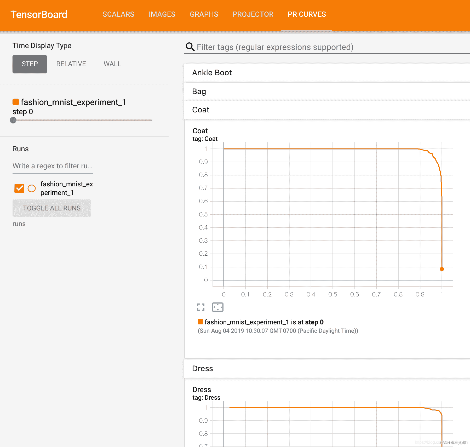
6.3.4 add_pr_curve to view the PR curve of each category

Reference 《Precision-Recall Curves》

Display the precision-recall curve (Prediction-Recall Curve).

add_pr_curve(tag, labels, predictions, global_step=None, num_thresholds=127,
    weights=None, walltime=None)

• labels: target value
• predictions: predicted values
• num_thresholds: Number of interpolation points in the middle of the curve
• weights: weight of each point

# 1\. gets the probability predictions in a test_size x num_classes Tensor
# 2\. gets the preds in a test_size Tensor
# takes ~10 seconds to run
class_probs = [] # 预测概率
class_preds = [] # 预测类别标签
with torch.no_grad():
    for data in testloader:
        images, labels = data
        output = net(images)
        class_probs_batch = [F.softmax(el, dim=0) for el in output]
        _, class_preds_batch = torch.max(output, 1)

        class_probs.append(class_probs_batch)
        class_preds.append(class_preds_batch)

test_probs = torch.cat([torch.stack(batch) for batch in class_probs])
test_preds = torch.cat(class_preds)

# helper function
def add_pr_curve_tensorboard(class_index, test_probs, test_preds, global_step=0):
    '''
    Takes in a "class_index" from 0 to 9 and plots the corresponding
    precision-recall curve
    '''
    tensorboard_preds = test_preds == class_index
    tensorboard_probs = test_probs[:, class_index]

    writer.add_pr_curve(classes[class_index],
                        tensorboard_preds,
                        tensorboard_probs,
                        global_step=global_step)
    writer.close()

# plot all the pr curves
for i in range(len(classes)):
    add_pr_curve_tensorboard(i, test_probs, test_preds)

  You will now see a "PR Curves" tab that contains the precision-recall curves for each category. Keep poking around; you'll notice that in some categories the model's "area under the curve" is close to 100%, and in others it's lower:

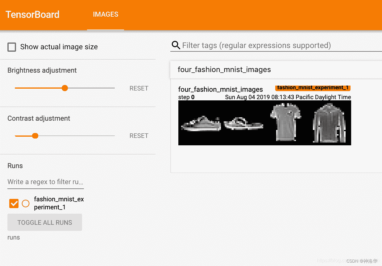
6.3.5 add_image writes pictures

# get some random training images
dataiter = iter(trainloader)
images, labels = dataiter.next()

# create grid of images
img_grid = torchvision.utils.make_grid(images)

# show images
matplotlib_imshow(img_grid, one_channel=True)

# write to tensorboard
writer.add_image('four_fashion_mnist_images', img_grid)
tensorboard --logdir=runs

6.3.6 Modify port

  Sometimes, in order to avoid colliding with other people's TensorBoard ports when training the model on the server, we need to specify a new port. Or sometimes when we run TensorBoard in a docker container, we map it to the host through a port. In this case, we need to specify TensorBoard to use a specific port. The format is: tensorboard --logdir=数据文件夹 --port=端口. For example:

tensorboard --logdir=./Feb05_01-00-48_Alienware/ --port=10000

6.3.7 Compare multiple running curves

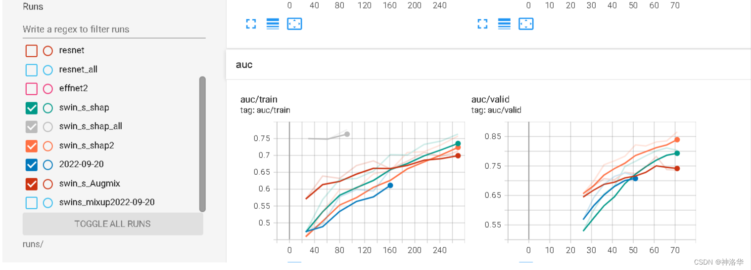
• When running by yourself, you need to experiment with various hyperparameters to find the optimal combination. It is tiring to run line by line every time to look at various loss and acc curves, and the effect is not good. TensorBoard can load multiple running results for comparison at a glance.
• It should be noted that if the log log is in a folder, the curves of other logs will only be displayed as the background and cannot be filtered, so you must select a different log_dir for each run . The same model will be run multiple times, and just naming it after the model name will not work, so consider adding time.

save_name=swins_mixup # 代表swin_transformer模型的S Type（一共有T、S、L三种模型大小），以及数据增强用了Mixup
board_time  = "{0:%Y-%m-%dT%H-%M-%S/}".format(datetime.now())
comment=f'save_nmae={
      
      save_name} lr={
      
      lr} transforms={
      
      transforms}' # 这个写了好像没啥用
writer = SummaryWriter(log_dir='runs/'+save_name+board_time,comment=comment)

run

%load_ext tensorboard
%tensorboard --logdir runs/

The backgrounds in the picture below are the curves displayed by different log files in the same folder. So when it comes to comparison, the logs cannot be in the same folder.

6.4 Use TensorBoard to check model architecture

One of TensorBoard's strengths is its ability to visualize complex model structures. Let's visualize the model we built.

writer.add_graph(net, images)
writer.close()

Now after refreshing TensorBoard, you should see a "Graphs" tab as shown below:

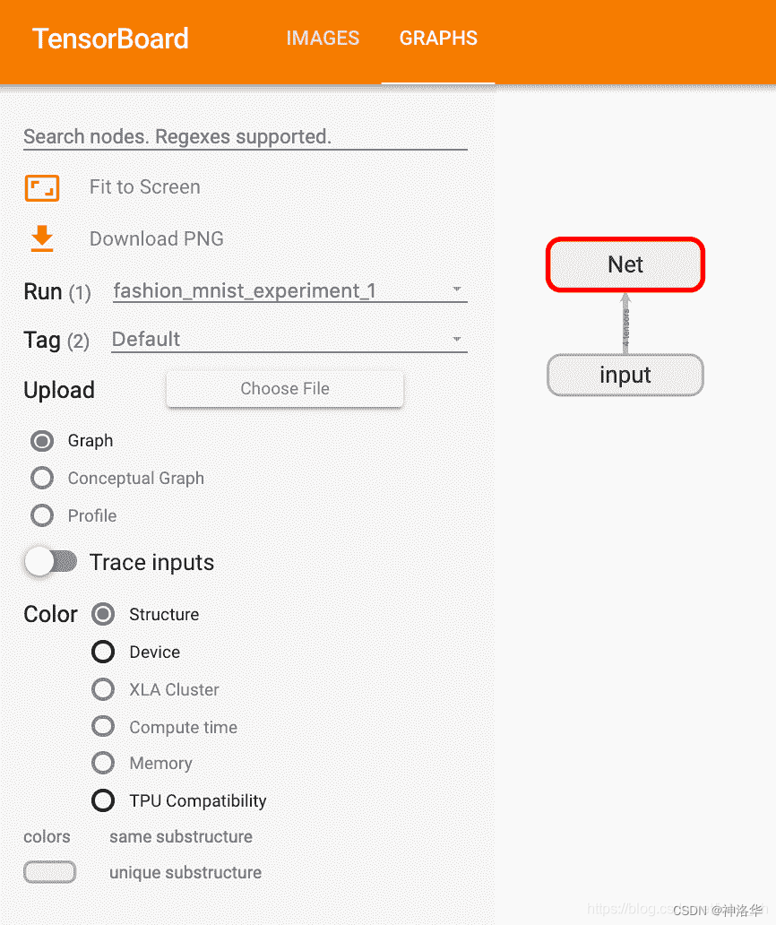
Go ahead and double-click "Net" to expand it to see a detailed view of the individual operations that make up the model.

6.5 add_embedding Visualize low-dimensional representation of high-dimensional data

TensorBoard has very convenient functions for visualizing high-dimensional data, such as image data, in a low-dimensional space; we will introduce it next.

# helper function
def select_n_random(data, labels, n=100):
    '''
    Selects n random datapoints and their corresponding labels from a dataset
    '''
    assert len(data) == len(labels)

    perm = torch.randperm(len(data))
    return data[perm][:n], labels[perm][:n]

# select random images and their target indices
images, labels = select_n_random(trainset.data, trainset.targets)

# get the class labels for each image
class_labels = [classes[lab] for lab in labels]

# log embeddings
features = images.view(-1, 28 * 28)
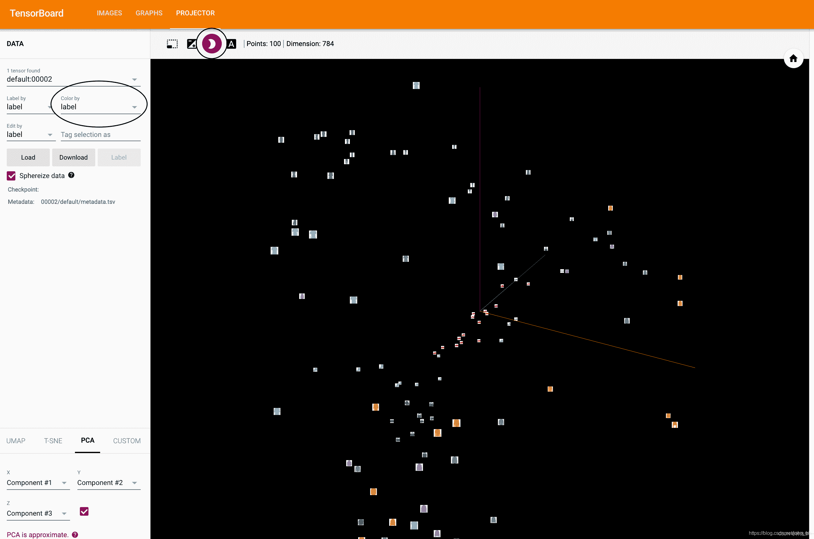
writer.add_embedding(features,
                    metadata=class_labels,
                    label_img=images.unsqueeze(1))
writer.close()

  Now, in TensorBoard's Projector tab, you can see these 100 images - 784 dimensions each - projected down into three-dimensional space. Furthermore, this is interactive: you can click and drag to rotate the 3D projection. Finally, there are two tricks to make the visualization easier to see: select "Color: Label" in the upper left, and enable "Night Mode", which will make the images easier to see since their background is white:

6.6 Track training and view model predictions through the plot_classes_preds function

# helper functions

def images_to_probs(net, images):
    '''
    Generates predictions and corresponding probabilities from a trained
    network and a list of images
    '''
    output = net(images)
    # convert output probabilities to predicted class
    _, preds_tensor = torch.max(output, 1)
    preds = np.squeeze(preds_tensor.numpy())
    return preds, [F.softmax(el, dim=0)[i].item() for i, el in zip(preds, output)]

def plot_classes_preds(net, images, labels):
    '''
    Generates matplotlib Figure using a trained network, along with images
    and labels from a batch, that shows the network's top prediction along
    with its probability, alongside the actual label, coloring this
    information based on whether the prediction was correct or not.
    Uses the "images_to_probs" function.
    '''
    preds, probs = images_to_probs(net, images)
    # plot the images in the batch, along with predicted and true labels
    fig = plt.figure(figsize=(12, 48))
    for idx in np.arange(4):
        ax = fig.add_subplot(1, 4, idx+1, xticks=[], yticks=[])
        matplotlib_imshow(images[idx], one_channel=True)
        ax.set_title("{0}, {1:.1f}%\n(label: {2})".format(
            classes[preds[idx]],
            probs[idx] * 100.0,
            classes[labels[idx]]),
                    color=("green" if preds[idx]==labels[idx].item() else "red"))
    return fig

During the training process, we will generate an image showing the model predictions and actual results for the four images contained in the batch.

running_loss = 0.0
for epoch in range(1):  # loop over the dataset multiple times

    for i, data in enumerate(trainloader, 0):

        # get the inputs; data is a list of [inputs, labels]
        inputs, labels = data

        # zero the parameter gradients
        optimizer.zero_grad()

        # forward + backward + optimize
        outputs = net(inputs)
        loss = criterion(outputs, labels)
        loss.backward()
        optimizer.step()

        running_loss += loss.item()
        if i % 1000 == 999:    # every 1000 mini-batches...

            # ...log the running loss
            writer.add_scalar('training loss',
                            running_loss / 1000,
                            epoch * len(trainloader) + i)

            # ...log a Matplotlib Figure showing the model's predictions on a
            # random mini-batch
            writer.add_figure('predictions vs. actuals',
                            plot_classes_preds(net, inputs, labels),
                            global_step=epoch * len(trainloader) + i)
            running_loss = 0.0
print('Finished Training')

  We can view the predictions made by the model on any batch throughout the learning process. Look at the "Images" tab and scroll down to see this under the "Predicted vs. Actual" visualization; this shows us that, for example, after only 3000 training iterations, the model is able to distinguish visually distinct categories such as shirts, sneakers and jackets

6.7 Introduction to tensorboard interface

The three on the upper right are:

• SCALARS: loss function image
• DISTRIBUTIONS: Weight distribution (over time)
• HISTOGRAMS: weighted histogram distribution

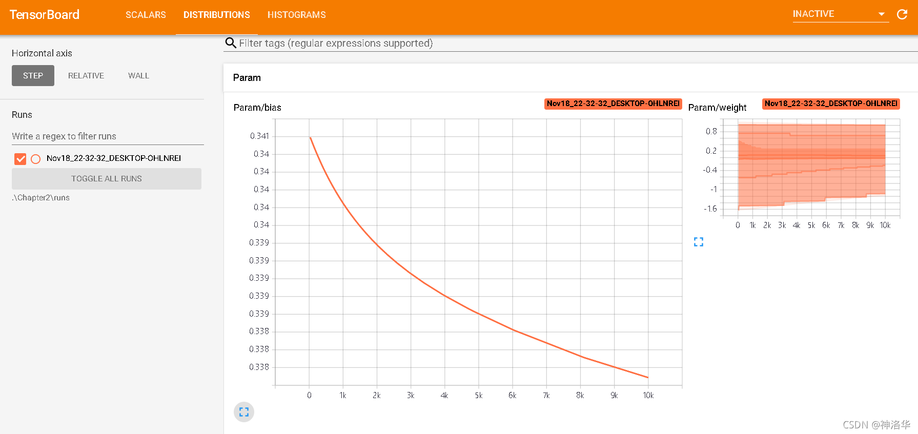
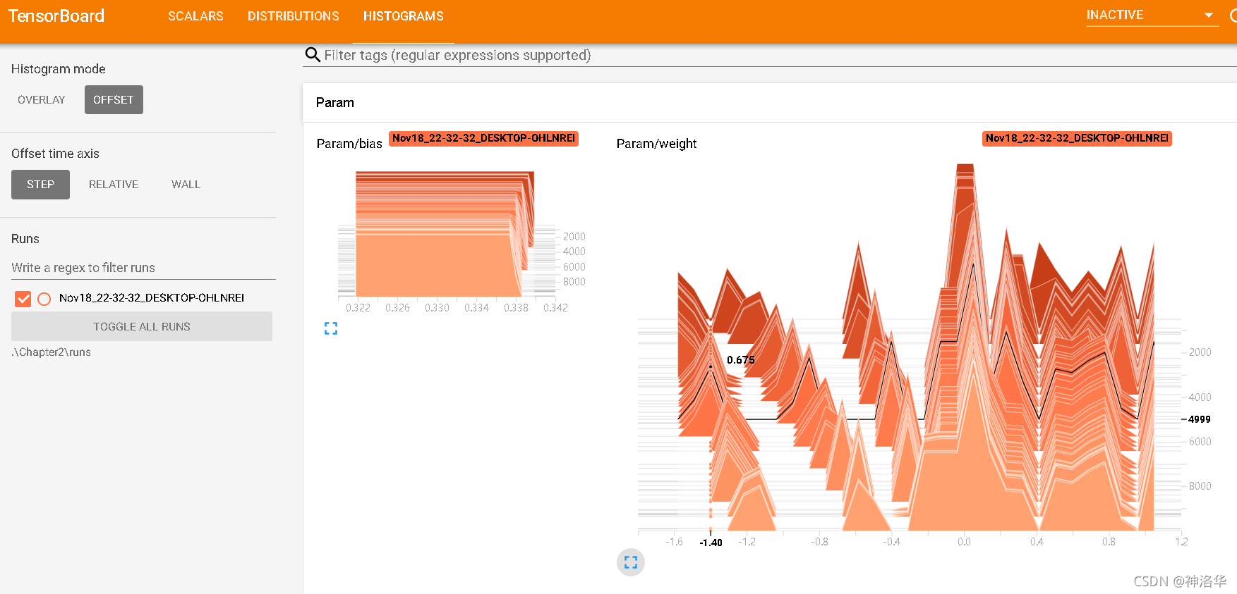
The weight distribution and histogram should change with training until the distribution stabilizes. If there is no change, there may be a problem with the model structure or backpropagation.

Scalars: This panel is the most commonly used panel. It is mainly used to draw the changes in acc (training set accuracy), val_acc (validation set accuracy), loss (loss value), weight (weight), etc. during the neural network training process. into a line chart.

• Ignore outlines in chart scaling (ignore outlines in chart scaling) can eliminate discrete values
• data downloadlinks: display data download links, used to download pictures
• Smoothing: The smoothness of the curve of the image. The larger the value, the smoother it is. The loss of each mini-batch does not necessarily decrease. The larger the smoothing is, the more mini-batches are on average.
• Horizontal Axis: Horizontal axis representation.
  • STEP: indicates the number of iterations
  • RELATIVE: represents the relative value between the training set and the test set
  • WALL: Indicates according to time.

7. Image conversion and augmentation

• Official document "Transforming and augmenting images"
• Refer to the post "Transforming and Augmenting Images" , data enhancement - Cutout, Random Erasing, Mixup, Cutmix

7.1 AUGMIX

参考《AUGMIX：A SIMPLE DATA PROCESSING METHOD TO IMPROVE ROBUSTNESS AND UNCERTA》

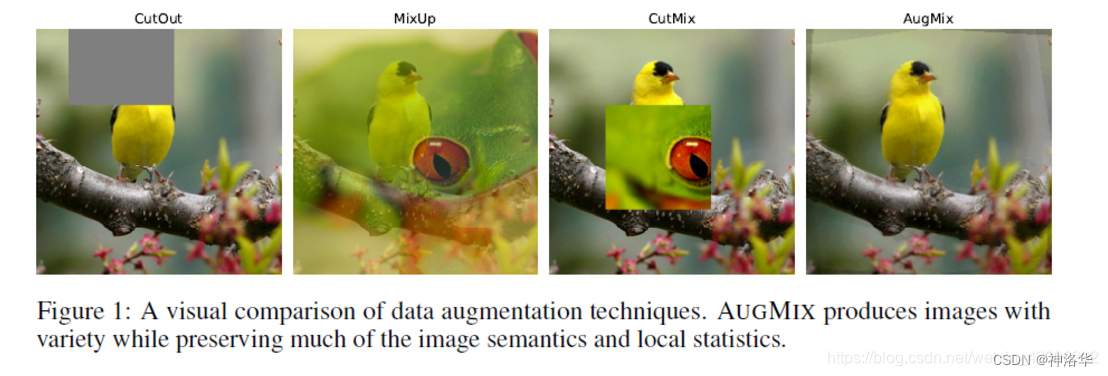
The latest proposed data augmentation methods include, as shown above:

1. CutOut: Randomly find a rectangular area on the picture and discard it.
2. MixUp: Fusion of pixels of two pictures according to a certain ratio. The fused picture has the labels of the two pictures.
3. CutMix: Similar to CutOut, the difference is that this rectangular area is filled with pixels from another picture. I personally tested it and found it to be stable and promising!
4. AugMix: Perform three parallel operations on an original image: transformation, rotation, and multi-tone, then merge it according to a certain ratio, and finally merge it with the original image according to a certain ratio. The operation is as follows: The approximate process is to perform k data on the original
   
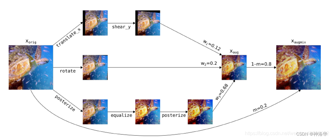
     image Augmentation operation, and then k weights are used to fuse to obtain the aug image. Finally, it is fused with the original image at a certain ratio to obtain the final augmentix image. The loss function Jensen-Shannon Divergence Consistency Loss is used in the paper to calculate the JS divergence between the augmented image and the original image. It is necessary to ensure the similarity between the augmented image and the original image.

7.2 Mixup

Refer to "mixup/cutout/Margin loss...simple implementation"

Mixup implementation:

!pip install torchtoolbox
from torchtoolbox.tools import mixup_data, mixup_criterion
 
alpha = 0.2
for i, (data, labels) in enumerate(train_data):
    data = data.to(device, non_blocking=True)
    labels = labels.to(device, non_blocking=True)
 
    data, labels_a, labels_b, lam = mixup_data(data, labels, alpha)
    optimizer.zero_grad()
    outputs = model(data)
    loss = mixup_criterion(Loss, outputs, labels_a, labels_b, lam)
 
    loss.backward()
    optimizer.update()

7.3 cutout/ArcLoss, CosLoss, L2Softmax

from torchvision import transforms
from torchtoolbox.transform import Cutout
 
train_transform = transforms.Compose([
    transforms.RandomResizedCrop(224),
    Cutout(),
    transforms.RandomHorizontalFlip(),
    transforms.ColorJitter(0.4, 0.4, 0.4),
    transforms.ToTensor(),
    normalize,
])

from torchtoolbox.nn.loss import ArcLoss, CosLoss, L2Softmax