
Article directory
Code link: https://github.com/open-mmlab/mmyolo/tree/main
Related documents:
1. The whole process of custom data set annotation + training + testing + deployment
2. Take you through the backbone network in 10 minutes
3. Easily master big picture reasoning in 10 minutes
5. Interpretation of configuration files
1. Introduction to MMYOLO
MMYOLO is an open source library for the YOLO series algorithms. The library supports one-time environment configuration and debugging of multiple models. Similar to other libraries in the MMLab series, it is a very useful library for learning and training the YOLO algorithm.
MMYOLO unifies the implementation of each YOLO algorithm module and provides a unified evaluation process. It decouples the YOLO algorithm into different module components. Custom models can be easily constructed by combining different modules and training strategies.
Algorithms supported by MMYOLO as of 2023.01.18:
- YOLOv5
- YOLOv6
- YOLOv7
- PPYOLOE
- RTMDet
- YOLOv8 (dev branch)
Many of the contents of this article are excerpted from the above official documents. For more detailed content, you need to consult the official documents yourself.
1.1 MMYOLO installation and simple training
conda create -n open-mmlab python=3.8 pytorch==1.10.1 torchvision==0.11.2 cudatoolkit=11.3 -c pytorch -y
conda activate open-mmlab
pip install openmim
mim install "mmengine>=0.3.1"
mim install "mmcv>=2.0.0rc1,<2.1.0"
mim install "mmdet>=3.0.0rc5,<3.1.0"
git clone https://github.com/open-mmlab/mmyolo.git
cd mmyolo
# Install albumentations
pip install -r requirements/albu.txt
# Install MMYOLO
mim install -v -e .
The code structure is as follows:
Download of MMYOLO data:
- COCO:
python tools/misc/download_dataset.py - Cat (comes with a small data set to facilitate experiments):
python tools/misc/download_dataset.py --dataset-name cat --unzip --delete --save-dir ./data/cat
train:
python tools/train.py configs/custom_dataset/yolov5_s-v61_syncbn_fast_1xb32-100e_cat.py
test:
python tools/test.py configs/custom_dataset/yolov5_s-v61_syncbn_fast_1xb32-100e_cat.py ./work_dirs/yolov6_s_syncbn_fast_1xb32-100e_cat/best_coco/bbox_mAP_epoch_96.pth
Visualization:
python demo/image_demo.py ./data/cat/images \
                          ./configs/custom_dataset/yolov6_s_syncbn_fast_1xb32-100e_cat.py \
                          ./work_dirs/yolov6_s_syncbn_fast_1xb32-100e_cat/best_coco/bbox_mAP_epoch_96.pth \
                          --out-dir ./data/cat/pred_images
deploy:
-
MMDeploy framework for deployment
-
Deploy using projects/easydeploy
1.2 Detailed configuration parameters
Training external parameters:
img_scale = (640, 640)            # 高度,宽度
deepen_factor = 0.33              # 控制网络结构深度的缩放因子,YOLOv5-s 为 0.33
widen_factor = 0.5                # 控制网络结构宽度的缩放因子,YOLOv5-s 为 0.5
max_epochs = 300                  # 最大训练轮次 300 轮
save_epoch_intervals = 10         # 验证间隔,每 10 个 epoch 验证一次
train_batch_size_per_gpu = 16     # 训练时单个 GPU 的 Batch size
train_num_workers = 8             # 训练时单个 GPU 分配的数据加载线程数
val_batch_size_per_gpu = 1        # 验证时单个 GPU 的 Batch size
val_num_workers = 2               # 验证时单个 GPU 分配的数据加载线程数
Model structure parameters:
- model: configure detection algorithm components
- backbone
- neck
- data_preprocessor
- train_cfg: training hyperparameters
- test_cfg: test hyperparameters
anchors = [[(10, 13), (16, 30), (33, 23)], # 多尺度的先验框基本尺寸
           [(30, 61), (62, 45), (59, 119)],
           [(116, 90), (156, 198), (373, 326)]]
strides = [8, 16, 32] # 先验框生成器的步幅

model = dict(
    type='YOLODetector', #检测器名
    data_preprocessor=dict(  # 数据预处理器的配置,通常包括图像归一化和 padding
        type='mmdet.DetDataPreprocessor',  # 数据预处理器的类型,还可以选择 'YOLOv5DetDataPreprocessor' 训练速度更快
        mean=[0., 0., 0.],  # 用于预训练骨干网络的图像归一化通道均值,按 R、G、B 排序
        std=[255., 255., 255.], # 用于预训练骨干网络的图像归一化通道标准差,按 R、G、B 排序
        bgr_to_rgb=True),  # 是否将图像通道从 BGR 转为 RGB
    backbone=dict(  # 主干网络的配置文件
        type='YOLOv5CSPDarknet',  # 主干网络的类别,目前可选用 'YOLOv5CSPDarknet', 'YOLOv6EfficientRep', 'YOLOXCSPDarknet' 3种
        deepen_factor=deepen_factor, # 控制网络结构深度的缩放因子
        widen_factor=widen_factor, # 控制网络结构宽度的缩放因子
        norm_cfg=dict(type='BN', momentum=0.03, eps=0.001), # 归一化层(norm layer)的配置项
        act_cfg=dict(type='SiLU', inplace=True)), # 激活函数(activation function)的配置项
    neck=dict(
        type='YOLOv5PAFPN',  # 检测器的 neck 是 YOLOv5FPN,我们同样支持 'YOLOv6RepPAFPN', 'YOLOXPAFPN'
        deepen_factor=deepen_factor, # 控制网络结构深度的缩放因子
        widen_factor=widen_factor, # 控制网络结构宽度的缩放因子
        in_channels=[256, 512, 1024], # 输入通道数,与 Backbone 的输出通道一致
        out_channels=[256, 512, 1024], # 输出通道数,与 Head 的输入通道一致
        num_csp_blocks=3, # CSPLayer 中 bottlenecks 的数量
        norm_cfg=dict(type='BN', momentum=0.03, eps=0.001), # 归一化层(norm layer)的配置项
        act_cfg=dict(type='SiLU', inplace=True)), # 激活函数(activation function)的配置项
    bbox_head=dict(
        type='YOLOv5Head', # bbox_head 的类型是 'YOLOv5Head', 我们目前也支持 'YOLOv6Head', 'YOLOXHead'
        head_module=dict(
            type='YOLOv5HeadModule', # head_module 的类型是 'YOLOv5HeadModule', 我们目前也支持 'YOLOv6HeadModule', 'YOLOXHeadModule'
            num_classes=80, # 分类的类别数量
            in_channels=[256, 512, 1024], # 输入通道数,与 Neck 的输出通道一致
            widen_factor=widen_factor, # 控制网络结构宽度的缩放因子
            featmap_strides=[8, 16, 32], # 多尺度特征图的步幅
            num_base_priors=3), # 在一个点上,先验框的数量
        prior_generator=dict( # 先验框(prior)生成器的配置
            type='mmdet.YOLOAnchorGenerator', # 先验框生成器的类型是 mmdet 中的 'YOLOAnchorGenerator'
            base_sizes=anchors, # 多尺度的先验框基本尺寸
            strides=strides), # 先验框生成器的步幅, 与 FPN 特征步幅一致。如果未设置 base_sizes,则当前步幅值将被视为 base_sizes。
    ),
    test_cfg=dict(
        multi_label=True, # 对于多类别预测来说是否考虑多标签,默认设置为 True
        nms_pre=30000,  # NMS 前保留的最大检测框数目
        score_thr=0.001, # 过滤类别的分值,低于 score_thr 的检测框当做背景处理
        nms=dict(type='nms', # NMS 的类型
                 iou_threshold=0.65), # NMS 的阈值
        max_per_img=300)) # 每张图像 NMS 后保留的最大检测框数目
There are differences between the training and test data streams of YOLOv5
1) YOLOv5 training data flow
dataset_type = 'CocoDataset'  # 数据集类型,这将被用来定义数据集
data_root = 'data/coco/'  # 数据的根路径
file_client_args = dict(backend='disk')  # 文件读取后端的配置,默认从硬盘读取

pre_transform = [ # 训练数据读取流程
    dict(
        type='LoadImageFromFile', # 第 1 个流程,从文件路径里加载图像
        file_client_args=file_client_args),  # 文件读取后端的配置,默认从硬盘读取
    dict(type='LoadAnnotations', # 第 2 个流程,对于当前图像,加载它的注释信息
         with_bbox=True) # 是否使用标注框(bounding box),目标检测需要设置为 True
]

albu_train_transforms = [                # YOLOv5-v6.1 仓库中,引入了 Albumentation 代码库进行图像的数据增广, 请确保其版本为 1.0.+
    dict(type='Blur', p=0.01),       # 图像模糊,模糊概率 0.01
    dict(type='MedianBlur', p=0.01), # 均值模糊,模糊概率 0.01
    dict(type='ToGray', p=0.01),         # 随机转换为灰度图像,转灰度概率 0.01
    dict(type='CLAHE', p=0.01)                 # CLAHE(限制对比度自适应直方图均衡化) 图像增强方法,直方图均衡化概率 0.01
]
train_pipeline = [                                # 训练数据处理流程
    *pre_transform,                                # 引入前述定义的训练数据读取流程
    dict(
        type='Mosaic',          # Mosaic 数据增强方法
        img_scale=img_scale,    # Mosaic 数据增强后的图像尺寸
        pad_val=114.0,          # 空区域填充像素值
        pre_transform=pre_transform), # 之前创建的 pre_transform 训练数据读取流程
    dict(
        type='YOLOv5RandomAffine',            # YOLOv5 的随机仿射变换
        max_rotate_degree=0.0,          # 最大旋转角度
        max_shear_degree=0.0,           # 最大错切角度
        scaling_ratio_range=(0.5, 1.5), # 图像缩放系数的范围
        border=(-img_scale[0] // 2, -img_scale[1] // 2), # 从输入图像的高度和宽度两侧调整输出形状的距离
        border_val=(114, 114, 114)), # 边界区域填充像素值
    dict(
        type='mmdet.Albu',                        # mmdet 中的 Albumentation 数据增强
        transforms=albu_train_transforms, # 之前创建的 albu_train_transforms 数据增强流程
        bbox_params=dict(
            type='BboxParams',
            format='pascal_voc',
            label_fields=['gt_bboxes_labels', 'gt_ignore_flags']),
        keymap={


            'img': 'image',
            'gt_bboxes': 'bboxes'
        }),
    dict(type='YOLOv5HSVRandomAug'),            # HSV通道随机增强
    dict(type='mmdet.RandomFlip', prob=0.5),        # 随机翻转,翻转概率 0.5
    dict(
        type='mmdet.PackDetInputs',                                # 将数据转换为检测器输入格式的流程
        meta_keys=('img_id', 'img_path', 'ori_shape', 'img_shape', 'flip',
                   'flip_direction'))
]
train_dataloader = dict( # 训练 dataloader 配置
    batch_size=train_batch_size_per_gpu, # 训练时单个 GPU 的 Batch size
    num_workers=train_num_workers, # 训练时单个 GPU 分配的数据加载线程数
    persistent_workers=True, # 如果设置为 True,dataloader 在迭代完一轮之后不会关闭数据读取的子进程,可以加速训练
    pin_memory=True, # 开启锁页内存,节省 CPU 内存拷贝时间
    sampler=dict( # 训练数据的采样器
        type='DefaultSampler', # 默认的采样器,同时支持分布式和非分布式训练。请参考 https://github.com/open-mmlab/mmengine/blob/main/mmengine/dataset/sampler.py
        shuffle=True), # 随机打乱每个轮次训练数据的顺序
    dataset=dict( # 训练数据集的配置
        type=dataset_type,
        data_root=data_root,
        ann_file='annotations/instances_train2017.json', # 标注文件路径
        data_prefix=dict(img='train2017/'), # 图像路径前缀
        filter_cfg=dict(filter_empty_gt=False, min_size=32), # 图像和标注的过滤配置
        pipeline=train_pipeline)) # 这是由之前创建的 train_pipeline 定义的数据处理流程
2) YOLOv5 test data flow
In the testing phase, the Letter Resize method is used to unify all test images to the same scale, thereby effectively retaining the aspect ratio of the images. Therefore, we use the same data flow for reasoning during verification and evaluation.
test_pipeline = [ # 测试数据处理流程
    dict(
        type='LoadImageFromFile', # 第 1 个流程,从文件路径里加载图像
        file_client_args=file_client_args),  # 文件读取后端的配置,默认从硬盘读取
    dict(type='YOLOv5KeepRatioResize', # 第 2 个流程,保持长宽比的图像大小缩放
         scale=img_scale), # 图像缩放的目标尺寸
    dict(
        type='LetterResize', # 第 3 个流程,满足多种步幅要求的图像大小缩放
        scale=img_scale, # 图像缩放的目标尺寸
        allow_scale_up=False, # 当 ratio > 1 时,是否允许放大图像,
        pad_val=dict(img=114)), # 空区域填充像素值
    dict(type='LoadAnnotations', with_bbox=True), # 第 4 个流程,对于当前图像,加载它的注释信息
    dict(
        type='mmdet.PackDetInputs', # 将数据转换为检测器输入格式的流程
        meta_keys=('img_id', 'img_path', 'ori_shape', 'img_shape',
                   'scale_factor', 'pad_param'))
]

val_dataloader = dict(
    batch_size=val_batch_size_per_gpu, # 验证时单个 GPU 的 Batch size
    num_workers=val_num_workers, # 验证时单个 GPU 分配的数据加载线程数
    persistent_workers=True, # 如果设置为 True,dataloader 在迭代完一轮之后不会关闭数据读取的子进程,可以加速训练
    pin_memory=True, # 开启锁页内存,节省 CPU 内存拷贝时间
    drop_last=False, # 是否丢弃最后未能组成一个批次的数据
    sampler=dict(
        type='DefaultSampler', # 默认的采样器,同时支持分布式和非分布式训练
        shuffle=False), # 验证和测试时不打乱数据顺序
    dataset=dict(
        type=dataset_type,
        data_root=data_root,
        test_mode=True, # 开启测试模式,避免数据集过滤图像和标注
        data_prefix=dict(img='val2017/'), # 图像路径前缀
        ann_file='annotations/instances_val2017.json', # 标注文件路径
        pipeline=test_pipeline, # 这是由之前创建的 test_pipeline 定义的数据处理流程
        batch_shapes_cfg=dict(  # batch shapes 配置
            type='BatchShapePolicy', # 确保在 batch 推理过程中同一个 batch 内的图像 pad 像素最少,不要求整个验证过程中所有 batch 的图像尺度一样
            batch_size=val_batch_size_per_gpu, # batch shapes 策略的 batch size,等于验证时单个 GPU 的 Batch size
            img_size=img_scale[0], # 图像的尺寸
            size_divisor=32, # padding 后的图像的大小应该可以被 pad_size_divisor 整除
            extra_pad_ratio=0.5))) # 额外需要 pad 的像素比例

test_dataloader = val_dataloader
3) Evaluation
The evaluator and dataset are decoupled in the OpenMMLab 2.0 version, so the new version design can easily implement VOC dataset using coco metric and other similar requirements.
val_evaluator = dict(  # 验证过程使用的评测器
    type='mmdet.CocoMetric',  # 用于评估检测的 AR、AP 和 mAP 的 coco 评价指标
    proposal_nums=(100, 1, 10),        # 用于评估检测任务时,选取的Proposal数量
    ann_file=data_root + 'annotations/instances_val2017.json',  # 标注文件路径
    metric='bbox',  # 需要计算的评价指标,`bbox` 用于检测
)
test_evaluator = val_evaluator  # 测试过程使用的评测器
Since the test data set does not have annotation files, the test_dataloader and test_evaluator configurations in MMYOLO are usually equal to val. If you want to save the detection results on the test data set, you can write the configuration like this:
# 在测试集上推理,
# 并将检测结果转换格式以用于提交结果
test_dataloader = dict(
    batch_size=1,
    num_workers=2,
    persistent_workers=True,
    drop_last=False,
    sampler=dict(type='DefaultSampler', shuffle=False),
    dataset=dict(
        type=dataset_type,
        data_root=data_root,
        ann_file=data_root + 'annotations/image_info_test-dev2017.json',
        data_prefix=dict(img='test2017/'),
        test_mode=True,
        pipeline=test_pipeline))
test_evaluator = dict(
    type='mmdet.CocoMetric',
    ann_file=data_root + 'annotations/image_info_test-dev2017.json',
    metric='bbox',
    format_only=True,  # 只将模型输出转换为coco的 JSON 格式并保存
    outfile_prefix='./work_dirs/coco_detection/test')  # 要保存的 JSON 文件的前缀
Configuration for training and testing:
MMEngine's Runner uses Loop to control training, verification and testing
You can use these fields to set the maximum training epochs and validation intervals
max_epochs = 300 # 最大训练轮次 300 轮
save_epoch_intervals = 10 # 验证间隔,每 10 轮验证一次

train_cfg = dict(
    type='EpochBasedTrainLoop',  # 训练循环的类型,请参考 https://github.com/open-mmlab/mmengine/blob/main/mmengine/runner/loops.py
    max_epochs=max_epochs,  # 最大训练轮次 300 轮
    val_interval=save_epoch_intervals)  # 验证间隔,每 10 个 epoch 验证一次
val_cfg = dict(type='ValLoop')  # 验证循环的类型
test_cfg = dict(type='TestLoop')  # 测试循环的类型
MMEngine also supports dynamic evaluation intervals. It can be verified every 10 epochs in the first 280 epoch training phase, and every 1 epoch in the last 20 epoch training. The configuration is written as:
max_epochs = 300 # 最大训练轮次 300 轮
save_epoch_intervals = 10 # 验证间隔,每 10 轮验证一次

train_cfg = dict(
    type='EpochBasedTrainLoop',  # 训练循环的类型,请参考 https://github.com/open-mmlab/mmengine/blob/main/mmengine/runner/loops.py
    max_epochs=max_epochs,  # 最大训练轮次 300 轮
    val_interval=save_epoch_intervals,  # 验证间隔,每 10 个 epoch 验证一次
    dynamic_intervals=[(280, 1)]) # 到 280 epoch 开始切换为间隔 1 的评估方式
val_cfg = dict(type='ValLoop')  # 验证循环的类型
test_cfg = dict(type='TestLoop')  # 测试循环的类型
1.3 Build the Config file of the Cat data set
_base_ = '../yolov5/yolov5_s-v61_syncbn_fast_8xb16-300e_coco.py'

max_epochs = 100  # 训练的最大 epoch
data_root = './data/cat/'  # 数据集目录的绝对路径
# data_root = '/root/workspace/mmyolo/data/cat/'  # Docker 容器里面数据集目录的绝对路径

# 结果保存的路径,可以省略,省略保存的文件名位于 work_dirs 下 config 同名的文件夹中
# 如果某个 config 只是修改了部分参数,修改这个变量就可以将新的训练文件保存到其他地方
work_dir = './work_dirs/yolov5_s-v61_syncbn_fast_1xb32-100e_cat'

# load_from 可以指定本地路径或者 URL,设置了 URL 会自动进行下载,因为上面已经下载过,我们这里设置本地路径
# 因为本教程是在 cat 数据集上微调,故这里需要使用 `load_from` 来加载 MMYOLO 中的预训练模型,这样可以在加快收敛速度的同时保证精度
load_from = './work_dirs/yolov5_s-v61_syncbn_fast_8xb16-300e_coco_20220918_084700-86e02187.pth'  # noqa

# 根据自己的 GPU 情况,修改 batch size,YOLOv5-s 默认为 8卡 x 16bs
train_batch_size_per_gpu = 32
train_num_workers = 4  # 推荐使用 train_num_workers = nGPU x 4

save_epoch_intervals = 2  # 每 interval 轮迭代进行一次保存一次权重

# 根据自己的 GPU 情况,修改 base_lr,修改的比例是 base_lr_default * (your_bs / default_bs)
base_lr = _base_.base_lr / 4

anchors = [  # 此处已经根据数据集特点更新了 anchor,关于 anchor 的生成,后面小节会讲解
    [(68, 69), (154, 91), (143, 162)],  # P3/8
    [(242, 160), (189, 287), (391, 207)],  # P4/16
    [(353, 337), (539, 341), (443, 432)]  # P5/32
]

class_name = ('cat', )  # 根据 class_with_id.txt 类别信息,设置 class_name
num_classes = len(class_name)
metainfo = dict(
    CLASSES=class_name, # 注意:这个字段在最新版本中换成了小写
    PALETTE=[(220, 20, 60)]  # 画图时候的颜色,随便设置即可
)

train_cfg = dict(
    max_epochs=max_epochs,
    val_begin=20,  # 第几个 epoch 后验证,这里设置 20 是因为前 20 个 epoch 精度不高,测试意义不大,故跳过
    val_interval=save_epoch_intervals  # 每 val_interval 轮迭代进行一次测试评估
)

model = dict(
    bbox_head=dict(
        head_module=dict(num_classes=num_classes),
        prior_generator=dict(base_sizes=anchors),

        # loss_cls 会根据 num_classes 动态调整,但是 num_classes = 1 的时候,loss_cls 恒为 0
        loss_cls=dict(loss_weight=0.5 *
                      (num_classes / 80 * 3 / _base_.num_det_layers))))

train_dataloader = dict(
    batch_size=train_batch_size_per_gpu,
    num_workers=train_num_workers,
    dataset=dict(
        _delete_=True,
        type='RepeatDataset',
        # 数据量太少的话,可以使用 RepeatDataset ,在每个 epoch 内重复当前数据集 n 次,这里设置 5 是重复 5 次
        times=5,
        dataset=dict(
            type=_base_.dataset_type,
            data_root=data_root,
            metainfo=metainfo,
            ann_file='annotations/trainval.json',
            data_prefix=dict(img='images/'),
            filter_cfg=dict(filter_empty_gt=False, min_size=32),
            pipeline=_base_.train_pipeline)))

val_dataloader = dict(
    dataset=dict(
        metainfo=metainfo,
        data_root=data_root,
        ann_file='annotations/trainval.json',
        data_prefix=dict(img='images/')))

test_dataloader = val_dataloader

val_evaluator = dict(ann_file=data_root + 'annotations/trainval.json')
test_evaluator = val_evaluator

optim_wrapper = dict(optimizer=dict(lr=base_lr))

default_hooks = dict(
    # 设置间隔多少个 epoch 保存模型,以及保存模型最多几个,`save_best` 是另外保存最佳模型(推荐)
    checkpoint=dict(
        type='CheckpointHook',
        interval=save_epoch_intervals,
        max_keep_ckpts=5,
        save_best='auto'),
    param_scheduler=dict(max_epochs=max_epochs),
    # logger 输出的间隔
    logger=dict(type='LoggerHook', interval=10))
1.3.1 Visualization of data set distribution
You can use MMYOLO's own data set visual analysis function to analyze the characteristics of different data sets, verify the correctness of the configuration file, and conduct preliminary analysis of the data set.
# 查看训练集的分布:
python tools/analysis_tools/dataset_analysis.py configs/custom_dataset/yolov5_s-v61_syncbn_fast_1xb32-100e_cat.py \
                                                --out-dir work_dirs/dataset_analysis_cat/train_dataset

# 查看验证集的分布:
python tools/analysis_tools/dataset_analysis.py configs/custom_dataset/yolov5_s-v61_syncbn_fast_1xb32-100e_cat.py \
                                                --out-dir work_dirs/dataset_analysis_cat/val_dataset \
                                                --val-dataset
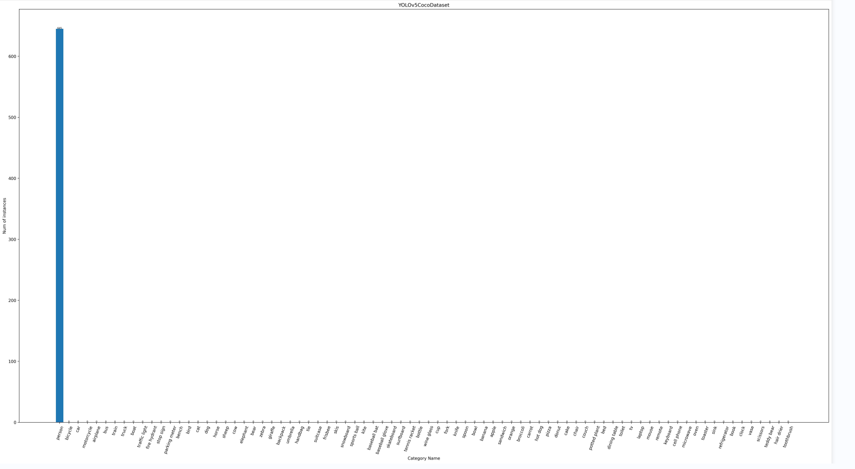
Training set information:
The category shown here is person, which should actually be cat. Don’t worry about this category. I just tried to run it here. The specific content is not debugged.
Print current running information:
+--------------------------------------------------------------------+
|                        Dataset information                         |
+---------------+-------------+--------------+-----------------------+
|  Dataset type |  Class name |   Function   |       Area rule       |
+---------------+-------------+--------------+-----------------------+
| train_dataset | All classes | All function | [0, 32, 96, 100000.0] |
+---------------+-------------+--------------+-----------------------+

Read the information of each picture in the dataset:
[>>>>>>>>>>>>>>>>>>>>>>>>>>>>>>>>>>>>>>>>>>>>>>] 580/580, 6437.8 task/s, elapsed: 0s, ETA:     0s

The information obtained is as follows:
+-------------------------------------------------------------------------------------------------               -------+
|                                      Information of dataset class                                                     |
+---------------+----------+----------------+----------+--------------+----------+------------+---               -------+
| Class name    | Bbox num | Class name     | Bbox num | Class name   | Bbox num | Class name | Bb               ox num |
+---------------+----------+----------------+----------+--------------+----------+------------+---               -------+
| person        | 645      | umbrella       | 0        | broccoli     | 0        | vase       | 0                       |
| bicycle       | 0        | handbag        | 0        | carrot       | 0        | scissors   | 0                       |
| car           | 0        | tie            | 0        | hot dog      | 0        | teddy bear | 0                       |
| motorcycle    | 0        | suitcase       | 0        | pizza        | 0        | hair drier | 0                       |
| airplane      | 0        | frisbee        | 0        | donut        | 0        | toothbrush | 0                       |
| bus           | 0        | skis           | 0        | cake         | 0        |            |                         |
| train         | 0        | snowboard      | 0        | chair        | 0        |            |                         |
| truck         | 0        | sports ball    | 0        | couch        | 0        |            |                         |
| boat          | 0        | kite           | 0        | potted plant | 0        |            |                         |
| traffic light | 0        | baseball bat   | 0        | bed          | 0        |            |                         |
| fire hydrant  | 0        | baseball glove | 0        | dining table | 0        |            |                         |
| stop sign     | 0        | skateboard     | 0        | toilet       | 0        |            |                         |
| parking meter | 0        | surfboard      | 0        | tv           | 0        |            |                         |
| bench         | 0        | tennis racket  | 0        | laptop       | 0        |            |                         |
| bird          | 0        | bottle         | 0        | mouse        | 0        |            |                         |
| cat           | 0        | wine glass     | 0        | remote       | 0        |            |                         |
| dog           | 0        | cup            | 0        | keyboard     | 0        |            |                         |
| horse         | 0        | fork           | 0        | cell phone   | 0        |            |                         |
| sheep         | 0        | knife          | 0        | microwave    | 0        |            |                         |
| cow           | 0        | spoon          | 0        | oven         | 0        |            |                         |
| elephant      | 0        | bowl           | 0        | toaster      | 0        |            |                         |
| bear          | 0        | banana         | 0        | sink         | 0        |            |                         |
| zebra         | 0        | apple          | 0        | refrigerator | 0        |            |                         |
| giraffe       | 0        | sandwich       | 0        | book         | 0        |            |                         |
| backpack      | 0        | orange         | 0        | clock        | 0        |            |                         |
+---------------+----------+----------------+----------+--------------+----------+------------+---               -------+
YOLOv5CocoDataset_bbox_num.jpg
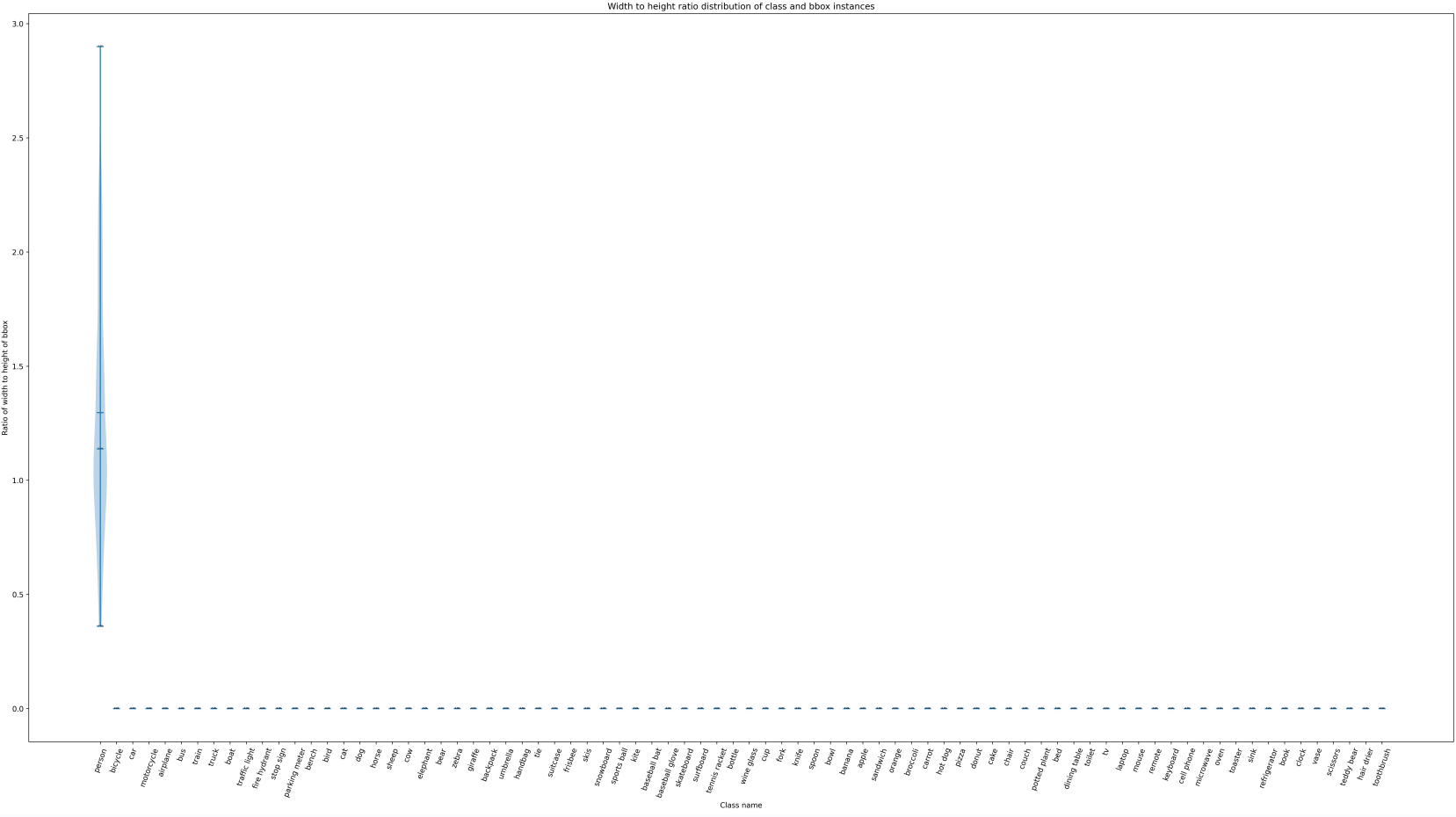
YOLOv5CocoDataset_bbox_ratio.jpg
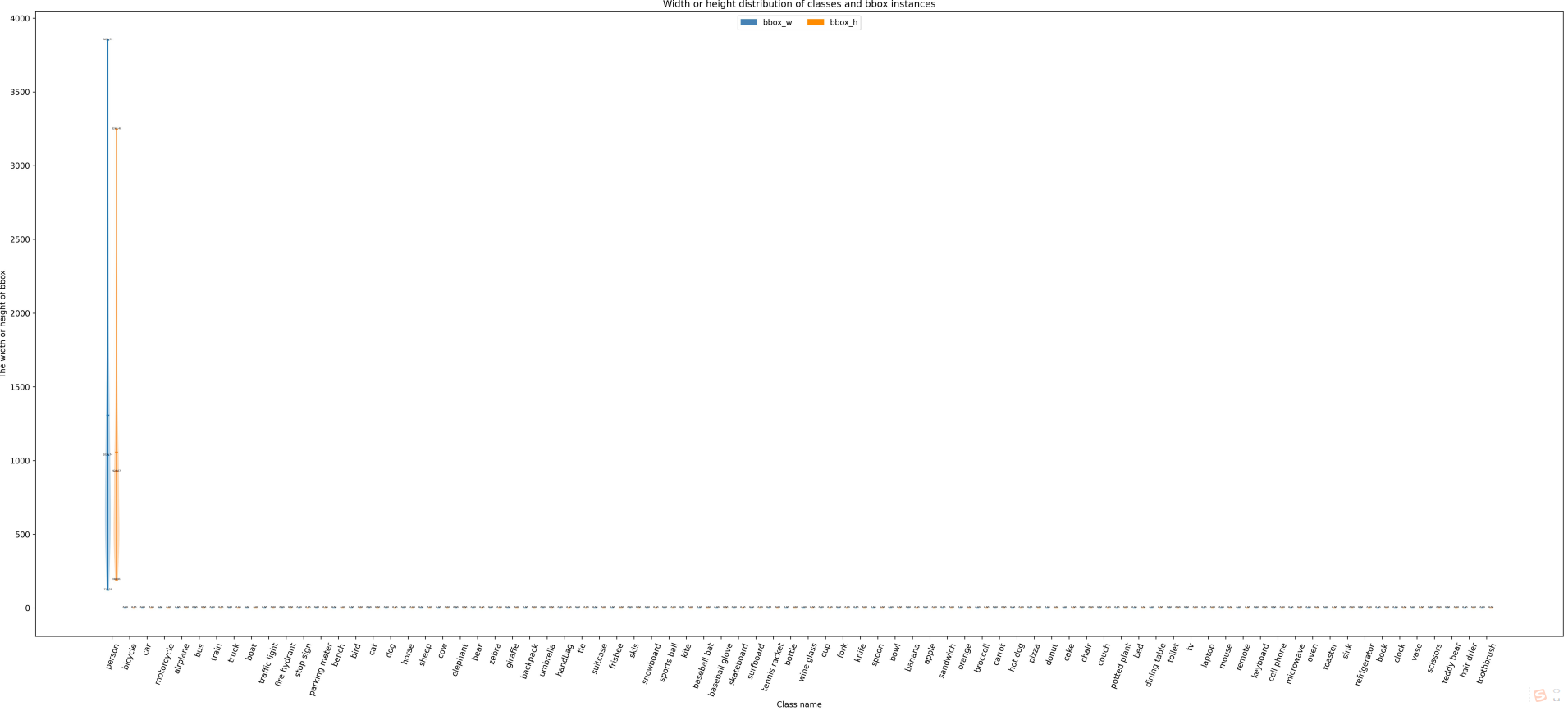
YOLOv5CocoDataset_bbox_wh.jpg
1.3.2 Optimization of anchor size in Anchor-based method
MMYOLO also supports optimizing the anchor size in the anchor-based method, and the anchor-free method can skip this step.
The script tools/analysis_tools/optimize_anchors.pysupports the following three anchor generation methods:
- k-means
- Differential Evolution
- v5-k-means
# 使用 yolov5-k-means 来进行优化的方式如下
python tools/analysis_tools/optimize_anchors.py configs/custom_dataset/yolov5_s-v61_syncbn_fast_1xb32-100e_cat.py \
                                                --algorithm v5-k-means \
                                                --input-shape 640 640 \
                                                --prior-match-thr 4.0 \
                                                --out-dir work_dirs/dataset_analysis_cat
You can modify the corresponding anchor size in the config according to the obtained anchor size.
It is worth noting that k-means is a clustering method, and there is a certain degree of randomness related to initialization, so the anchor obtained after each execution will be slightly different, but they are all generated based on the data set, so there will not be a big difference Influence.
Let’s briefly introduce the above three different anchor generation methods:
1)k-means
2)Differential Evolution
3)v5-k-means
1.3.3 Visual data processing
The script tools/analysis_tools/browse_dataset.py can help users directly visualize the data processing part of the config configuration, and can choose to save the visual image to a specified folder.
Use the trained model and the corresponding config file to visualize the pictures, pop up the display, each picture takes 3 seconds, and does not save:
python tools/analysis_tools/browse_dataset.py configs/custom_dataset/yolov5_s-v61_syncbn_fast_1xb32-100e_cat.py \
                                              --show-interval 3
2. Framework structure of MMYOLO
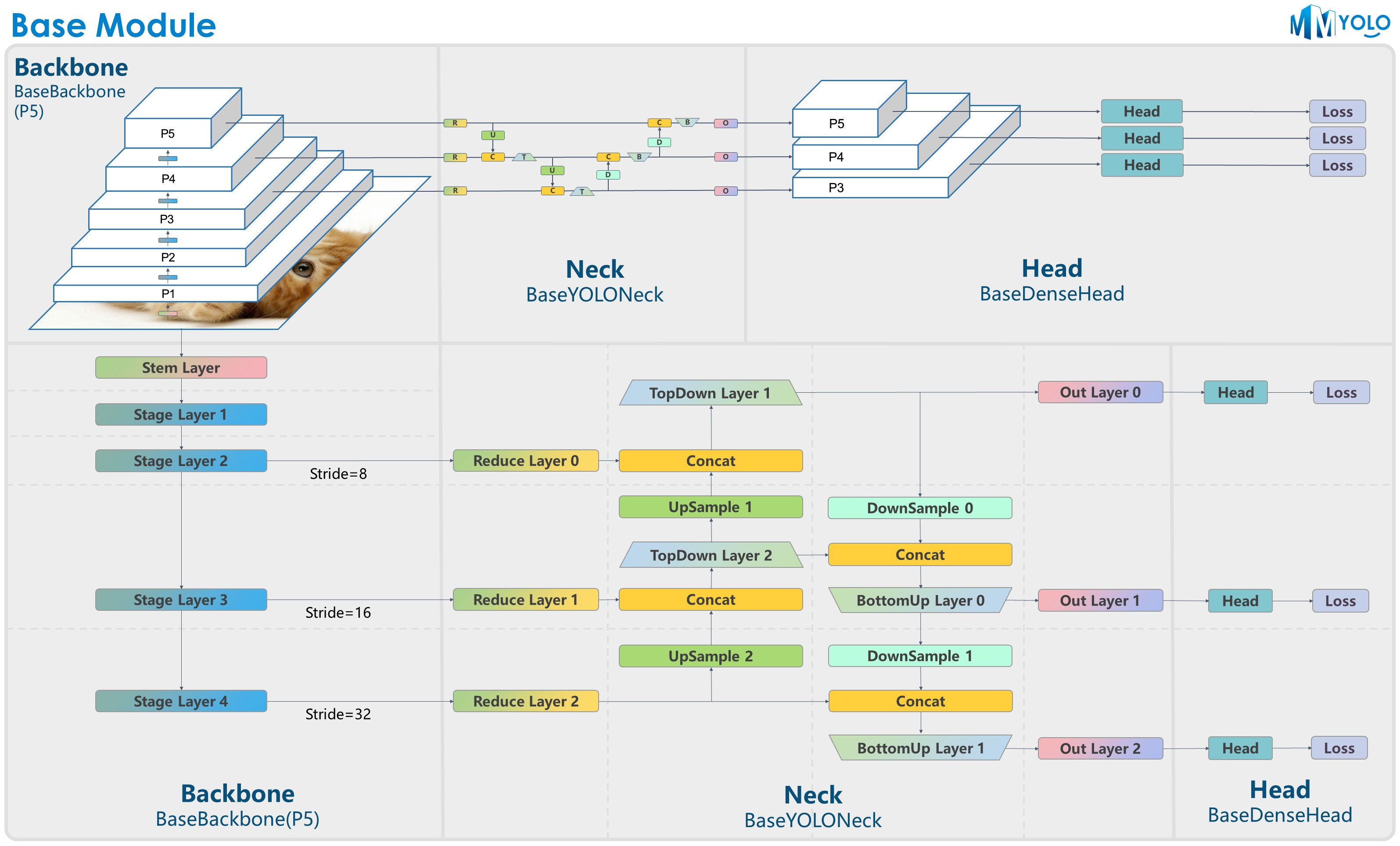
The core of MMYOLO is in the mmyolo library
MMYOLO divides the YOLO method into the following modules:
- datasets: supports various data sets for target detection
- transforms: Contains various data enhancement transformations
- models: Contains the various components that make up the model
- data_preprocessors: input data for preprocessing models
- detectors: define the desired detection model class
- Backbone:base_backbone / cps_darknet / csp_resnet / cspnext / efficient_rep / yolov7_backbone
- Neck:base_yolo_neck / cspnext_pafpn / yolov5_fpn / yolov6_fpn / yolov7_fpn / yolox_fpn
- Head:yolov5_head / yolov6_head / yolov7_head / yolox_head / ppyoloe_head / rtmdet_head
- Loss: various loss functions
- task_modules:assigners、samplers、box coders、prior generators
- layers: basic layers of neural network
- engine: part of the runtime component
- optimizer: optimizer
- hooks: runner hook
2.1 Take YOLOv5 as an example to illustrate the framework structure of MMYOLO
The organization method of MMYOLO is still: Backbone, Neck, Head
The YOLOv5 mentioned here is the v6.0 version, there is no Focus, it is replaced by conv, and SPPF is used instead of SPP.
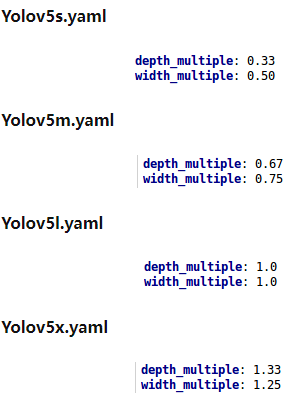
There are 4 versions of the YOLOv5 model, namely:
- YOLOv5s: The smallest depth and width (the latter gradually increase)
- YOLOv5m
- YOLOv5l
- YOLOv5x
The framework structure of YOLOv5 is as follows:
- Bckbone:CSPDarkNet
- Neck:PA-FPN
- Head: three scales, 3 types of anchors placed on each feature point of each scale
The YOLOv5 model framework is as follows:
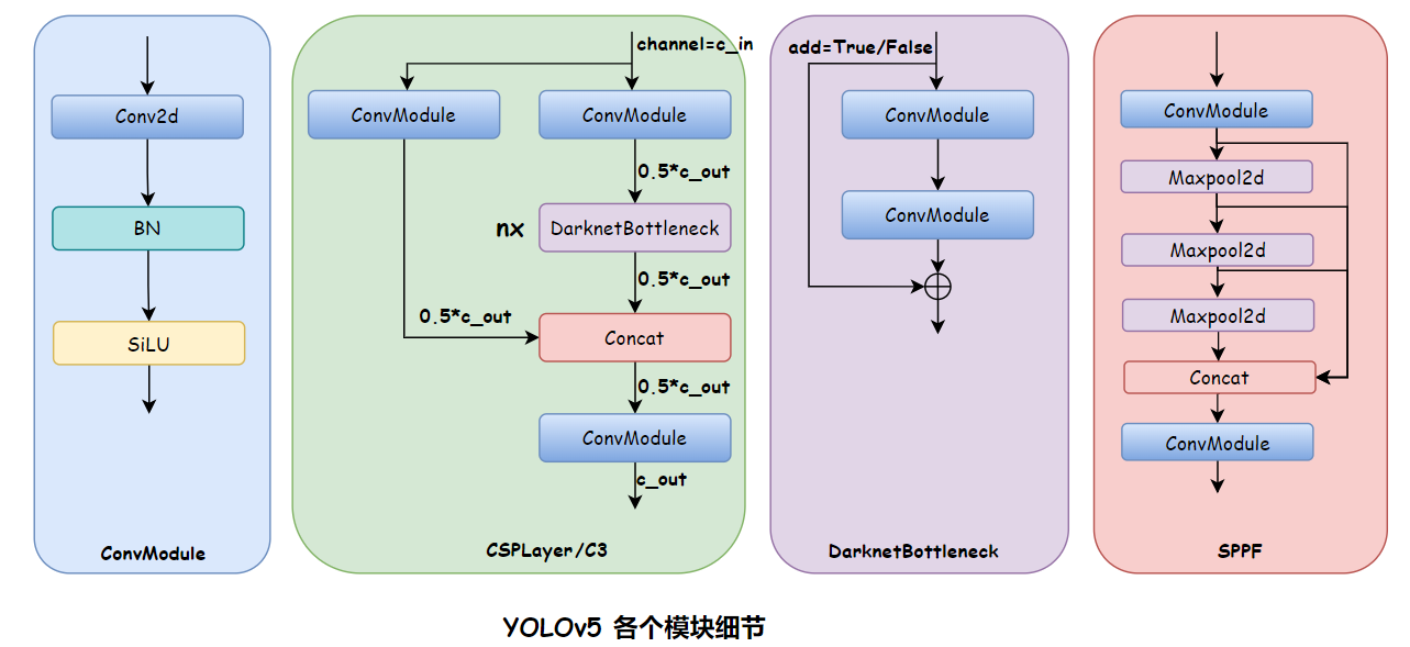
YOLOv5 module details are as follows:
2.1.1 Backbone
CSPDarkNet
The model content of YOLOv5-s's config is as follows:
deepen_factor = 0.33
widen_factor = 0.5
model = dict(
    type='YOLODetector',
    data_preprocessor=dict(
        type='mmdet.DetDataPreprocessor',
        mean=[0., 0., 0.],
        std=[255., 255., 255.],
        bgr_to_rgb=True),
    backbone=dict(
        type='YOLOv5CSPDarknet',
        deepen_factor=deepen_factor,
        widen_factor=widen_factor,
        norm_cfg=dict(type='BN', momentum=0.03, eps=0.001),
        act_cfg=dict(type='SiLU', inplace=True)),
    neck=dict(
        type='YOLOv5PAFPN',
        deepen_factor=deepen_factor,
        widen_factor=widen_factor,
        in_channels=[256, 512, 1024],
        out_channels=[256, 512, 1024],
        num_csp_blocks=3,
        norm_cfg=dict(type='BN', momentum=0.03, eps=0.001),
        act_cfg=dict(type='SiLU', inplace=True)),
    bbox_head=dict(
        type='YOLOv5Head',
        head_module=dict(
            type='YOLOv5HeadModule',
            num_classes=num_classes,
            in_channels=[256, 512, 1024],
            widen_factor=widen_factor,
            featmap_strides=strides,
            num_base_priors=3),
        prior_generator=dict(
            type='mmdet.YOLOAnchorGenerator',
            base_sizes=anchors,
            strides=strides),
        # scaled based on number of detection layers
        loss_cls=dict(
            type='mmdet.CrossEntropyLoss',
            use_sigmoid=True,
            reduction='mean',
            loss_weight=0.5 * (num_classes / 80 * 3 / num_det_layers)),
        loss_bbox=dict(
            type='IoULoss',
            iou_mode='ciou',
            bbox_format='xywh',
            eps=1e-7,
            reduction='mean',
            loss_weight=0.05 * (3 / num_det_layers),
            return_iou=True),
        loss_obj=dict(
            type='mmdet.CrossEntropyLoss',
            use_sigmoid=True,
            reduction='mean',
            loss_weight=1.0 * ((img_scale[0] / 640)**2 * 3 / num_det_layers)),
        prior_match_thr=4.,
        obj_level_weights=[4., 1., 0.4]),
    test_cfg=dict(
        multi_label=True,
        nms_pre=30000,
        score_thr=0.001,
        nms=dict(type='nms', iou_threshold=0.65),
        max_per_img=300))
YOLOv5 framework structure:
How to view the model structure:
tools/train.pyPut a breakpoint after line 109:
    else:
        # build customized runner from the registry
        # if 'runner_type' is set in the cfg
        runner = RUNNERS.build(cfg)
    import pdb; pdb.set_trace()
    # start training
    runner.train()
Then enter in the terminal runner.modelto get the structure of the model. Since the model is too long, I will briefly summarize it here:
YOLODetector(
  (data_preprocessor): YOLOv5DetDataPreprocessor()
  (backbone): YOLOv5CSPDarknet()
  (neck): YOLOv5PAFPN()
  (bbox_head): YOLOv5Head()
)
Backboneas follows:
 (backbone): YOLOv5CSPDarknet(
    (stem): conv(in=3, out=32, size=6x6, s=2, pading=2) + BN + SiLU
    (stage1): conv(in=32, out=64, size=3X3, s=2, pading=1) + BN + SiLU
    		  CSPLayer:conv(in=64, out=32, size=1x1, s=1) + BN + SiLU
    		  		   conv(in=64, out=32, size=1x1, s=1) + BN + SiLU
    		  		   conv(in=64, out=64, size=1x1, s=1) + BN + SiLU
    		  		   DarknetBottleNeck0:conv(in=32, out=32, size=1x1, s=1) + BN + SiLU
    		  		   					 conv(in=32, out=32, size=3x3, s=1, padding=1) + BN + SiLU
    (stage2): conv(in=64, out=128, size=3X3, s=2, pading=1) + BN + SiLU
    		  CSPLayer:conv(in=128, out=64, size=1x1, s=1) + BN + SiLU
    		  		   conv(in=128, out=64, size=1x1, s=1) + BN + SiLU
    		  		   conv(in=128, out=128, size=1x1, s=1) + BN + SiLU
    		  		   DarknetBottleNeck0:conv(in=64, out=64, size=1x1, s=1) + BN + SiLU
    		  		   					  conv(in=64, out=64, size=3x3, s=1, padding=1) + BN + SiLU
		  		   	   DarknetBottleNeck1:conv(in=64, out=64, size=1x1, s=1) + BN + SiLU
		  		   					      conv(in=64, out=64, size=3x3, s=1, padding=1) + BN + SiLU
    (stage3): conv(in=128, out=256, size=3X3, s=2, pading=1) + BN + SiLU
    		  CSPLayer:conv(in=256, out=128, size=1x1, s=1) + BN + SiLU
    		  		   conv(in=256, out=128, size=1x1, s=1) + BN + SiLU
    		  		   conv(in=256, out=128, size=1x1, s=1) + BN + SiLU
    		  		   DarknetBottleNeck0:conv(in=128, out=128, size=1x1, s=1) + BN + SiLU
    		  		   					  conv(in=128, out=128, size=3x3, s=1, padding=1) + BN + SiLU
		  		   	   DarknetBottleNeck1:conv(in=128, out=128, size=1x1, s=1) + BN + SiLU
		  		   					      conv(in=128, out=128, size=3x3, s=1, padding=1) + BN + SiLU
		  		   	   DarknetBottleNeck2:conv(in=128, out=128, size=1x1, s=1) + BN + SiLU
		  		   					      conv(in=128, out=128, size=3x3, s=1, padding=1) + BN + SiLU
    (stage4): conv(in=256, out=512, size=3X3, s=2, pading=1) + BN + SiLU
    		  CSPLayer:conv(in=512, out=256, size=1x1, s=1) + BN + SiLU
    		  		   conv(in=512, out=256, size=1x1, s=1) + BN + SiLU
    		  		   conv(in=512, out=512, size=1x1, s=1) + BN + SiLU
    		  		   DarknetBottleNeck0:conv(in=256, out=256, size=1x1, s=1) + BN + SiLU
    		  		   					  conv(in=256, out=256, size=3x3, s=1, padding=1) + BN + SiLU
 		   	  SPPF:conv(in=512, out=256, size=1x1, s=1) + BN + SiLU
 		   	       maxpooling(size=5x5, s=1, padding=2, dilation=1)
 		   		   conv(in=1024, out=512, size=1x1, s=1, padding=1) + BN + SiLU
The entire model framework structure is as follows:
 (backbone): YOLOv5CSPDarknet(
    (stem): ConvModule(
      (conv): Conv2d(3, 32, kernel_size=(6, 6), stride=(2, 2), padding=(2, 2), bias=False)
      (bn): BatchNorm2d(32, eps=0.001, momentum=0.03, affine=True, track_running_stats=True)
      (activate): SiLU(inplace=True)
    )
    (stage1): Sequential(
      (0): ConvModule(
        (conv): Conv2d(32, 64, kernel_size=(3, 3), stride=(2, 2), padding=(1, 1), bias=False)
        (bn): BatchNorm2d(64, eps=0.001, momentum=0.03, affine=True, track_running_stats=True)
        (activate): SiLU(inplace=True)
      )
      (1): CSPLayer(
        (main_conv): ConvModule(
          (conv): Conv2d(64, 32, kernel_size=(1, 1), stride=(1, 1), bias=False)
          (bn): BatchNorm2d(32, eps=0.001, momentum=0.03, affine=True, track_running_stats=True)
          (activate): SiLU(inplace=True)
        )
        (short_conv): ConvModule(
          (conv): Conv2d(64, 32, kernel_size=(1, 1), stride=(1, 1), bias=False)
          (bn): BatchNorm2d(32, eps=0.001, momentum=0.03, affine=True, track_running_stats=True)
          (activate): SiLU(inplace=True)
        )
        (final_conv): ConvModule(
          (conv): Conv2d(64, 64, kernel_size=(1, 1), stride=(1, 1), bias=False)
          (bn): BatchNorm2d(64, eps=0.001, momentum=0.03, affine=True, track_running_stats=True)
          (activate): SiLU(inplace=True)
        )
        (blocks): Sequential(
          (0): DarknetBottleneck(
            (conv1): ConvModule(
              (conv): Conv2d(32, 32, kernel_size=(1, 1), stride=(1, 1), bias=False)
              (bn): BatchNorm2d(32, eps=0.001, momentum=0.03, affine=True, track_running_stats=True)
              (activate): SiLU(inplace=True)
            )
            (conv2): ConvModule(
              (conv): Conv2d(32, 32, kernel_size=(3, 3), stride=(1, 1), padding=(1, 1), bias=False)
              (bn): BatchNorm2d(32, eps=0.001, momentum=0.03, affine=True, track_running_stats=True)
              (activate): SiLU(inplace=True)
            )
          )
        )
      )
    )
    (stage2): Sequential(
      (0): ConvModule(
        (conv): Conv2d(64, 128, kernel_size=(3, 3), stride=(2, 2), padding=(1, 1), bias=False)
        (bn): BatchNorm2d(128, eps=0.001, momentum=0.03, affine=True, track_running_stats=True)
        (activate): SiLU(inplace=True)
      )
      (1): CSPLayer(
        (main_conv): ConvModule(
          (conv): Conv2d(128, 64, kernel_size=(1, 1), stride=(1, 1), bias=False)
          (bn): BatchNorm2d(64, eps=0.001, momentum=0.03, affine=True, track_running_stats=True)
          (activate): SiLU(inplace=True)
        )
        (short_conv): ConvModule(
          (conv): Conv2d(128, 64, kernel_size=(1, 1), stride=(1, 1), bias=False)
          (bn): BatchNorm2d(64, eps=0.001, momentum=0.03, affine=True, track_running_stats=True)
          (activate): SiLU(inplace=True)
        )
        (final_conv): ConvModule(
          (conv): Conv2d(128, 128, kernel_size=(1, 1), stride=(1, 1), bias=False)
          (bn): BatchNorm2d(128, eps=0.001, momentum=0.03, affine=True, track_running_stats=True)
          (activate): SiLU(inplace=True)
        )
        (blocks): Sequential(
          (0): DarknetBottleneck(
            (conv1): ConvModule(
              (conv): Conv2d(64, 64, kernel_size=(1, 1), stride=(1, 1), bias=False)
              (bn): BatchNorm2d(64, eps=0.001, momentum=0.03, affine=True, track_running_stats=True)
              (activate): SiLU(inplace=True)
            )
            (conv2): ConvModule(
              (conv): Conv2d(64, 64, kernel_size=(3, 3), stride=(1, 1), padding=(1, 1), bias=False)
              (bn): BatchNorm2d(64, eps=0.001, momentum=0.03, affine=True, track_running_stats=True)
              (activate): SiLU(inplace=True)
            )
          )
          (1): DarknetBottleneck(
            (conv1): ConvModule(
              (conv): Conv2d(64, 64, kernel_size=(1, 1), stride=(1, 1), bias=False)
              (bn): BatchNorm2d(64, eps=0.001, momentum=0.03, affine=True, track_running_stats=True)
              (activate): SiLU(inplace=True)
            )
            (conv2): ConvModule(
              (conv): Conv2d(64, 64, kernel_size=(3, 3), stride=(1, 1), padding=(1, 1), bias=False)
              (bn): BatchNorm2d(64, eps=0.001, momentum=0.03, affine=True, track_running_stats=True)
              (activate): SiLU(inplace=True)
            )
          )
        )
      )
    )
    (stage3): Sequential(
      (0): ConvModule(
        (conv): Conv2d(128, 256, kernel_size=(3, 3), stride=(2, 2), padding=(1, 1), bias=False)
        (bn): BatchNorm2d(256, eps=0.001, momentum=0.03, affine=True, track_running_stats=True)
        (activate): SiLU(inplace=True)
      )
      (1): CSPLayer(
        (main_conv): ConvModule(
          (conv): Conv2d(256, 128, kernel_size=(1, 1), stride=(1, 1), bias=False)
          (bn): BatchNorm2d(128, eps=0.001, momentum=0.03, affine=True, track_running_stats=True)
          (activate): SiLU(inplace=True)
        )
        (short_conv): ConvModule(
          (conv): Conv2d(256, 128, kernel_size=(1, 1), stride=(1, 1), bias=False)
          (bn): BatchNorm2d(128, eps=0.001, momentum=0.03, affine=True, track_running_stats=True)
          (activate): SiLU(inplace=True)
        )
        (final_conv): ConvModule(
          (conv): Conv2d(256, 256, kernel_size=(1, 1), stride=(1, 1), bias=False)
          (bn): BatchNorm2d(256, eps=0.001, momentum=0.03, affine=True, track_running_stats=True)
          (activate): SiLU(inplace=True)
        )
        (blocks): Sequential(
          (0): DarknetBottleneck(
            (conv1): ConvModule(
              (conv): Conv2d(128, 128, kernel_size=(1, 1), stride=(1, 1), bias=False)
              (bn): BatchNorm2d(128, eps=0.001, momentum=0.03, affine=True, track_running_stats=True)
              (activate): SiLU(inplace=True)
            )
            (conv2): ConvModule(
              (conv): Conv2d(128, 128, kernel_size=(3, 3), stride=(1, 1), padding=(1, 1), bias=False)
              (bn): BatchNorm2d(128, eps=0.001, momentum=0.03, affine=True, track_running_stats=True)
              (activate): SiLU(inplace=True)
            )
          )
          (1): DarknetBottleneck(
            (conv1): ConvModule(
              (conv): Conv2d(128, 128, kernel_size=(1, 1), stride=(1, 1), bias=False)
              (bn): BatchNorm2d(128, eps=0.001, momentum=0.03, affine=True, track_running_stats=True)
              (activate): SiLU(inplace=True)
            )
            (conv2): ConvModule(
              (conv): Conv2d(128, 128, kernel_size=(3, 3), stride=(1, 1), padding=(1, 1), bias=False)
              (bn): BatchNorm2d(128, eps=0.001, momentum=0.03, affine=True, track_running_stats=True)
              (activate): SiLU(inplace=True)
            )
          )
          (2): DarknetBottleneck(
            (conv1): ConvModule(
              (conv): Conv2d(128, 128, kernel_size=(1, 1), stride=(1, 1), bias=False)
              (bn): BatchNorm2d(128, eps=0.001, momentum=0.03, affine=True, track_running_stats=True)
              (activate): SiLU(inplace=True)
            )
            (conv2): ConvModule(
              (conv): Conv2d(128, 128, kernel_size=(3, 3), stride=(1, 1), padding=(1, 1), bias=False)
              (bn): BatchNorm2d(128, eps=0.001, momentum=0.03, affine=True, track_running_stats=True)
              (activate): SiLU(inplace=True)
            )
          )
        )
      )
    )
    (stage4): Sequential(
      (0): ConvModule(
        (conv): Conv2d(256, 512, kernel_size=(3, 3), stride=(2, 2), padding=(1, 1), bias=False)
        (bn): BatchNorm2d(512, eps=0.001, momentum=0.03, affine=True, track_running_stats=True)
        (activate): SiLU(inplace=True)
      )
      (1): CSPLayer(
        (main_conv): ConvModule(
          (conv): Conv2d(512, 256, kernel_size=(1, 1), stride=(1, 1), bias=False)
          (bn): BatchNorm2d(256, eps=0.001, momentum=0.03, affine=True, track_running_stats=True)
          (activate): SiLU(inplace=True)
        )
        (short_conv): ConvModule(
          (conv): Conv2d(512, 256, kernel_size=(1, 1), stride=(1, 1), bias=False)
          (bn): BatchNorm2d(256, eps=0.001, momentum=0.03, affine=True, track_running_stats=True)
          (activate): SiLU(inplace=True)
        )
        (final_conv): ConvModule(
          (conv): Conv2d(512, 512, kernel_size=(1, 1), stride=(1, 1), bias=False)
          (bn): BatchNorm2d(512, eps=0.001, momentum=0.03, affine=True, track_running_stats=True)
          (activate): SiLU(inplace=True)
        )
        (blocks): Sequential(
          (0): DarknetBottleneck(
            (conv1): ConvModule(
              (conv): Conv2d(256, 256, kernel_size=(1, 1), stride=(1, 1), bias=False)
              (bn): BatchNorm2d(256, eps=0.001, momentum=0.03, affine=True, track_running_stats=True)
              (activate): SiLU(inplace=True)
            )
            (conv2): ConvModule(
              (conv): Conv2d(256, 256, kernel_size=(3, 3), stride=(1, 1), padding=(1, 1), bias=False)
              (bn): BatchNorm2d(256, eps=0.001, momentum=0.03, affine=True, track_running_stats=True)
              (activate): SiLU(inplace=True)
            )
          )
        )
      )
      (2): SPPFBottleneck(
        (conv1): ConvModule(
          (conv): Conv2d(512, 256, kernel_size=(1, 1), stride=(1, 1), bias=False)
          (bn): BatchNorm2d(256, eps=0.001, momentum=0.03, affine=True, track_running_stats=True)
          (activate): SiLU(inplace=True)
        )
        (poolings): MaxPool2d(kernel_size=5, stride=1, padding=2, dilation=1, ceil_mode=False)
        (conv2): ConvModule(
          (conv): Conv2d(1024, 512, kernel_size=(1, 1), stride=(1, 1), bias=False)
          (bn): BatchNorm2d(512, eps=0.001, momentum=0.03, affine=True, track_running_stats=True)
          (activate): SiLU(inplace=True)
        )
      )
    )
  )
  (neck): YOLOv5PAFPN(
    (reduce_layers): ModuleList(
      (0): Identity()
      (1): Identity()
      (2): ConvModule(
        (conv): Conv2d(512, 256, kernel_size=(1, 1), stride=(1, 1), bias=False)
        (bn): BatchNorm2d(256, eps=0.001, momentum=0.03, affine=True, track_running_stats=True)
        (activate): SiLU(inplace=True)
      )
    )
    (upsample_layers): ModuleList(
      (0): Upsample(scale_factor=2.0, mode=nearest)
      (1): Upsample(scale_factor=2.0, mode=nearest)
    )
    (top_down_layers): ModuleList(
      (0): Sequential(
        (0): CSPLayer(
          (main_conv): ConvModule(
            (conv): Conv2d(512, 128, kernel_size=(1, 1), stride=(1, 1), bias=False)
            (bn): BatchNorm2d(128, eps=0.001, momentum=0.03, affine=True, track_running_stats=True)
            (activate): SiLU(inplace=True)
          )
          (short_conv): ConvModule(
            (conv): Conv2d(512, 128, kernel_size=(1, 1), stride=(1, 1), bias=False)
            (bn): BatchNorm2d(128, eps=0.001, momentum=0.03, affine=True, track_running_stats=True)
            (activate): SiLU(inplace=True)
          )
          (final_conv): ConvModule(
            (conv): Conv2d(256, 256, kernel_size=(1, 1), stride=(1, 1), bias=False)
            (bn): BatchNorm2d(256, eps=0.001, momentum=0.03, affine=True, track_running_stats=True)
            (activate): SiLU(inplace=True)
          )
          (blocks): Sequential(
            (0): DarknetBottleneck(
              (conv1): ConvModule(
                (conv): Conv2d(128, 128, kernel_size=(1, 1), stride=(1, 1), bias=False)
                (bn): BatchNorm2d(128, eps=0.001, momentum=0.03, affine=True, track_running_stats=True)
                (activate): SiLU(inplace=True)
              )
              (conv2): ConvModule(
                (conv): Conv2d(128, 128, kernel_size=(3, 3), stride=(1, 1), padding=(1, 1), bias=False)
                (bn): BatchNorm2d(128, eps=0.001, momentum=0.03, affine=True, track_running_stats=True)
                (activate): SiLU(inplace=True)
              )
            )
          )
        )
        (1): ConvModule(
          (conv): Conv2d(256, 128, kernel_size=(1, 1), stride=(1, 1), bias=False)
          (bn): BatchNorm2d(128, eps=0.001, momentum=0.03, affine=True, track_running_stats=True)
          (activate): SiLU(inplace=True)
        )
      )
      (1): CSPLayer(
        (main_conv): ConvModule(
          (conv): Conv2d(256, 64, kernel_size=(1, 1), stride=(1, 1), bias=False)
          (bn): BatchNorm2d(64, eps=0.001, momentum=0.03, affine=True, track_running_stats=True)
          (activate): SiLU(inplace=True)
        )
        (short_conv): ConvModule(
          (conv): Conv2d(256, 64, kernel_size=(1, 1), stride=(1, 1), bias=False)
          (bn): BatchNorm2d(64, eps=0.001, momentum=0.03, affine=True, track_running_stats=True)
          (activate): SiLU(inplace=True)
        )
        (final_conv): ConvModule(
          (conv): Conv2d(128, 128, kernel_size=(1, 1), stride=(1, 1), bias=False)
          (bn): BatchNorm2d(128, eps=0.001, momentum=0.03, affine=True, track_running_stats=True)
          (activate): SiLU(inplace=True)
        )
        (blocks): Sequential(
          (0): DarknetBottleneck(
            (conv1): ConvModule(
              (conv): Conv2d(64, 64, kernel_size=(1, 1), stride=(1, 1), bias=False)
              (bn): BatchNorm2d(64, eps=0.001, momentum=0.03, affine=True, track_running_stats=True)
              (activate): SiLU(inplace=True)
            )
            (conv2): ConvModule(
              (conv): Conv2d(64, 64, kernel_size=(3, 3), stride=(1, 1), padding=(1, 1), bias=False)
              (bn): BatchNorm2d(64, eps=0.001, momentum=0.03, affine=True, track_running_stats=True)
              (activate): SiLU(inplace=True)
            )
          )
        )
      )
    )
    (downsample_layers): ModuleList(
      (0): ConvModule(
        (conv): Conv2d(128, 128, kernel_size=(3, 3), stride=(2, 2), padding=(1, 1), bias=False)
        (bn): BatchNorm2d(128, eps=0.001, momentum=0.03, affine=True, track_running_stats=True)
        (activate): SiLU(inplace=True)
      )
      (1): ConvModule(
        (conv): Conv2d(256, 256, kernel_size=(3, 3), stride=(2, 2), padding=(1, 1), bias=False)
        (bn): BatchNorm2d(256, eps=0.001, momentum=0.03, affine=True, track_running_stats=True)
        (activate): SiLU(inplace=True)
      )
    )
    (bottom_up_layers): ModuleList(
      (0): CSPLayer(
        (main_conv): ConvModule(
          (conv): Conv2d(256, 128, kernel_size=(1, 1), stride=(1, 1), bias=False)
          (bn): BatchNorm2d(128, eps=0.001, momentum=0.03, affine=True, track_running_stats=True)
          (activate): SiLU(inplace=True)
        )
        (short_conv): ConvModule(
          (conv): Conv2d(256, 128, kernel_size=(1, 1), stride=(1, 1), bias=False)
          (bn): BatchNorm2d(128, eps=0.001, momentum=0.03, affine=True, track_running_stats=True)
          (activate): SiLU(inplace=True)
        )
        (final_conv): ConvModule(
          (conv): Conv2d(256, 256, kernel_size=(1, 1), stride=(1, 1), bias=False)
          (bn): BatchNorm2d(256, eps=0.001, momentum=0.03, affine=True, track_running_stats=True)
          (activate): SiLU(inplace=True)
        )
        (blocks): Sequential(
          (0): DarknetBottleneck(
            (conv1): ConvModule(
              (conv): Conv2d(128, 128, kernel_size=(1, 1), stride=(1, 1), bias=False)
              (bn): BatchNorm2d(128, eps=0.001, momentum=0.03, affine=True, track_running_stats=True)
              (activate): SiLU(inplace=True)
            )
            (conv2): ConvModule(
              (conv): Conv2d(128, 128, kernel_size=(3, 3), stride=(1, 1), padding=(1, 1), bias=False)
              (bn): BatchNorm2d(128, eps=0.001, momentum=0.03, affine=True, track_running_stats=True)
              (activate): SiLU(inplace=True)
            )
          )
        )
      )
      (1): CSPLayer(
        (main_conv): ConvModule(
          (conv): Conv2d(512, 256, kernel_size=(1, 1), stride=(1, 1), bias=False)
          (bn): BatchNorm2d(256, eps=0.001, momentum=0.03, affine=True, track_running_stats=True)
          (activate): SiLU(inplace=True)
        )
        (short_conv): ConvModule(
          (conv): Conv2d(512, 256, kernel_size=(1, 1), stride=(1, 1), bias=False)
          (bn): BatchNorm2d(256, eps=0.001, momentum=0.03, affine=True, track_running_stats=True)
          (activate): SiLU(inplace=True)
        )
        (final_conv): ConvModule(
          (conv): Conv2d(512, 512, kernel_size=(1, 1), stride=(1, 1), bias=False)
          (bn): BatchNorm2d(512, eps=0.001, momentum=0.03, affine=True, track_running_stats=True)
          (activate): SiLU(inplace=True)
        )
        (blocks): Sequential(
          (0): DarknetBottleneck(
            (conv1): ConvModule(
              (conv): Conv2d(256, 256, kernel_size=(1, 1), stride=(1, 1), bias=False)
              (bn): BatchNorm2d(256, eps=0.001, momentum=0.03, affine=True, track_running_stats=True)
              (activate): SiLU(inplace=True)
            )
            (conv2): ConvModule(
              (conv): Conv2d(256, 256, kernel_size=(3, 3), stride=(1, 1), padding=(1, 1), bias=False)
              (bn): BatchNorm2d(256, eps=0.001, momentum=0.03, affine=True, track_running_stats=True)
              (activate): SiLU(inplace=True)
            )
          )
        )
      )
    )
    (out_layers): ModuleList(
      (0): Identity()
      (1): Identity()
      (2): Identity()
    )
  )
    (bbox_head): YOLOv5Head(
    (head_module): YOLOv5HeadModule(
      (convs_pred): ModuleList(
        (0): Conv2d(128, 18, kernel_size=(1, 1), stride=(1, 1))
        (1): Conv2d(256, 18, kernel_size=(1, 1), stride=(1, 1))
        (2): Conv2d(512, 18, kernel_size=(1, 1), stride=(1, 1))
      )
    )
    (loss_cls): CrossEntropyLoss(avg_non_ignore=False)
    (loss_bbox): IoULoss()
    (loss_obj): CrossEntropyLoss(avg_non_ignore=False)
  )
)
2.1.2 Neck
CSP-PAFPN
SPP and SPPF:
- SPP: Spatial Pyramid Poolig, which is spatial pyramid pooling. Pooling methods of different sizes are used in parallel, and then the resulting maxpooling output feature map is concated.
- SPPF: Spatial Pyramid Poolig Fast is a fast version of spatial pyramid pooling. The amount of calculation is reduced. It uses a serial method. The next maxpooling receives the output of the previous maxpooling, and then concats the output of all maxpooling.
import time
import torch
import torch.nn as nn


class SPP(nn.Module):
    def __init__(self):
        super().__init__()
        self.maxpool1 = nn.MaxPool2d(5, 1, padding=2)
        self.maxpool2 = nn.MaxPool2d(9, 1, padding=4)
        self.maxpool3 = nn.MaxPool2d(13, 1, padding=6)

    def forward(self, x):
        o1 = self.maxpool1(x)
        o2 = self.maxpool2(x)
        o3 = self.maxpool3(x)
        return torch.cat([x, o1, o2, o3], dim=1)


class SPPF(nn.Module):
    def __init__(self):
        super().__init__()
        self.maxpool = nn.MaxPool2d(5, 1, padding=2)

    def forward(self, x):
        o1 = self.maxpool(x)
        o2 = self.maxpool(o1)
        o3 = self.maxpool(o2)
        return torch.cat([x, o1, o2, o3], dim=1)
2.1.3 Head
The output of YOLOv5 is as follows:
- 80x80x((5+Ncls)x3): Each feature point has 4 regs, 1 confidence level, and Ncls category scores
- 40x40x((5+Ncls)x3)
- 20x20x((5+Ncls)x3)
anchor in YOLOv5:
# coco 初始设定 anchor 的宽高如下,每个尺度的 head 上放置 3 种 anchor
anchors:
  - [10,13, 16,30, 33,23]  # P3/8
  - [30,61, 62,45, 59,119]  # P4/16
  - [116,90, 156,198, 373,326]  # P5/32
How to place anchor:
- For each feature point on the 8x downsampled feature map (80x80), three types of anchors with width and height of (10, 13), (16, 30), and (33,23) are placed.
- For each feature point on the 16x downsampling feature map (40x40), three types of anchors with width and height of (30, 61), (62, 45), and (59, 119) are placed.
- For each feature point on the 32x downsampling feature map (20x20), three types of anchors with width and height of (116, 90), (156, 198), and (373,326) are placed.
2.2 How the YOLO series algorithms distribute positive and negative samples
How the YOLO series of algorithms allocate positive and negative anchors:
- The original idea of YOLO is which feature point the center point of the gt box falls into (actually the grid in v1), which feature point (the feature point on the head feature map can be regarded as a grid of the original image) is responsible for prediction The gt
- In YOLOv1, each feature point inputs 2 prediction boxes (7x7 size). During training, the IoU of these two prediction boxes and gt is calculated, and the prediction box with the larger IoU is retained as the final prediction box for the feature point. During inference The box with the larger score (the possibility of containing the object) is retained as the prediction box, and a result vector of 7x7x (5x2+80) is obtained. That is, the anchor with the largest IoU of gt is used as a positive sample, and the rest are used as negative samples.
- In YOLOv2, the k-means method is used to generate 5 anchors for each feature point (feature map size 13x13), calculate the IoU of the anchor on the feature point and the gt whose center falls into the feature point, and assign a sum to each gt The anchor with the largest IoU is used as a positive sample, and the anchor with an IoU smaller than the set threshold (such as 0.2) is used as a negative sample.
- In YOLOv3, similar to YOLOv2, the k-means method is used to generate 9 anchors for each feature point (feature map size 13x13, 26x26, 52x52), there are 3 anchors at each scale, the max_iou method is still used, and each gt is allocated An anchor with the largest IoU is used as a positive sample, and an anchor whose IoU is less than the set threshold (such as 0.2) is used as a negative sample.
- In YOLOv4, if the max_iou method is used to allocate only one positive sample to each gt, it may also lead to the missed detection of some targets. Therefore, in YOLOv4, anchor boxes whose IoU of general and gt are greater than the threshold are regarded as positive samples, and those with IoU less than the threshold are regarded as positive samples. Set the threshold as a negative sample
- In YOLOv5, a feature point will be divided into four quadrants, which of the four quadrants the center point of the gt is located in, and the two adjacent feature points will also be used as positive samples. If gt is biased towards the lower right quadrant, the right and lower feature points of the grid where gt is located will also be used as positive samples.
- In YOLOv6, TAL was introduced to allocate positive and negative samples. TAL introduced a measure of alignment between classification and regression: anchor alignment metric t = s α × u β t = s^{\alpha} \times u^{\ beta}t=sa×uβ , where s is the classification score, u is the IoU value, for each gt, select m anchors with the largest t values as positive samples, and other anchors as negative samples, and embed t into the classification and regression loss functions to achieve dynamic allocation . L cls = Σ i = 1 N pos ∣ ti ^ − si ∣ BCE ( si , ti ^ ) + Σ j = 1 N negsj γ BCE ( sj , 0 ) L_{cls} = \Sigma_{i=1}^{ N_{pos}} | \hat{t_i}-s_i|\ BCE(s_i, \hat{t_i}) +\Sigma_{j=1}^{N_{neg}}s_j^{\gamma}\ BCE(s_j , 0)Lcls=Si=1Npos∣ti^−si∣ BCE(si,ti^)+Sj=1Nnegsjc BCE(sj,0), L r e g = Σ i = 1 N p o s t i ^ L G I o U ( b i , b i ^ ) L_{reg} = \Sigma_{i=1}^{N_{pos}}\ \hat{t_i} \ L_{GIoU}(b_i, \hat{b_i}) Lreg=Si=1Npos ti^ LG I o U(bi,bi^) , the total training loss of TAL isL cls + L reg L_{cls}+L_{reg}Lcls+Lreg
- In YOLOv7, YOLOv5 is combined with SimOTA used in YOLOX, and the first step in SimOTA "using central prior" is replaced by the quadrant selection strategy in YOLOv5. (SimOTA: Find the transmission cost of each true value and anchor. For each true value, select the top k anchors with the smallest cost in the center area as the positive samples of the gt).
- In YOLOv8, TAL is also used
