OpenVINS official documentation part one

Reference link: OpenVINS https://docs.openvins.com/index.html

---

1. Getting Started

  Welcome to the OpenVIINS project! The following guide will help new users download the software and run it on our supported datasets. Additionally, we provide information on how to run your own sensors on our systems and provide guidance on how we calibrate them. If you see anything missing or need clarification, please feel free to ask questions.

High-level overview
  At a high level, the system is built on several key algorithms. We have ov_core at its core, which contains many standard computer vision algorithms and utilities that anyone can use. Specifically, it stores the following large components:

• Sparse feature visual tracking (based on KLT and descriptors)
• Basic mathematical types used to represent states
• Initialization process
• Multi-sensor simulator that generates synthetic measurements

  The ov_core library is used by the ov_msckf system that contains our filter-based estimators . Among them we have state,managers, type systems, prediction and update algorithms. We encourage users to review the specific documentation to learn more about what we offer. The ov_eval library has a bunch of evaluation methods and scripts that can be used to generate research results for publication.

1.5 Sensor Calibration—How to Calibrate Your Own Visual Inertial Sensor

Visual Inertial Sensor
  Someone may ask why use visual inertial sensor? The main reason is because of the complementarity of the two different sensing methods. The camera provides high-density external measurements of the environment, while the IMU measures the internal self-motion of the sensor platform. The IMU is crucial to provide robustness to the estimator while also providing system scaling in the case of a monocular camera.
  However, there are some challenges when utilizing IMUs in estimation. The IMU needs to estimate other bias terms, and high-precision calibration between the camera and IMU is required. Additionally, small errors in relative timestamps between sensors can degrade performance very quickly in dynamic trajectories. In this OpenVINS project, we address these issues by advocating online estimation of these extrinsic and temporal offset parameters between the camera and IMU.

Camera intrinsic parameter calibration (offline)
  The first task is to calibrate the camera intrinsic parameters, such as focal length, camera center and distortion parameters. Our team frequently uses the Kalibr calibration toolbox for offline calibration of internal and external parameters by performing the following steps:

1. Download and build the Kalibr toolbox.
2. Print out the calibration plate to be used (we usually use Aprilgrid 6x6 0.8x0.8 meters ).
3. Make sure sensor drivers are published to ROS with the correct timestamps.
4. Sensor preparation.
   ● Limit motion blur by reducing exposure time;
   ● Publish at a low frame rate to allow for larger differences in the data set (2-5hz); ●
   Make sure the calibration plate can be seen in the image;
   ● Make sure your sensor is in focus (can Use its kalibr_camera_focus or manually)
5. Record ROS packets and ensure that the calibration plate can be seen from different directions, distances and each part of the image plane. You can move the calibration plate and keep the camera still, or you can move the camera and keep the calibration plate still.
6. Finally run the calibration.
   ● Use kalibr_calibrate_cameras with the specified topic ● Depending on the degree of distortion, use pinhole-equi
   for fisheye , or pinhole-radtan if distortion is low
7. Check the final results and pay close attention to the final reprojection error plot, a good calibration has less than <0.2-0.5 pixel reprojection error.

IMU Intrinsic Calibration (Offline)
  Another intrinsic calibration is to calculate the inertial sensor intrinsic noise characteristics, which is required for batch optimization to calibrate the camera to the IMU transform and any VINS estimator so that we can correctly probabilistically fuse the image and inertial readings . Unfortunately, there is no mature open source toolbox to find these values, instead try our kalibr_allan project, although it is not optimized. Specifically, we estimate the following noise parameters:

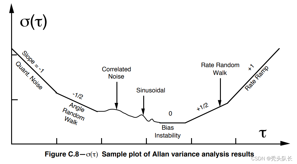
  As shown in the figure above, if we calculate the Allen variance, we can see that on the left side of the figure $t=1$ and fit this line with -1/2 slope to obtain the white noise of the sensor. Similarly, one can evaluate the right side$t=3$ and 1/2 slope of this line to obtain random walk noise. We have a package that can do this in matlab, but the actual verification and conversion to a C++ codebase is not yet complete. See ourkalibr_allangithub project for details on how to generate this plot and calculate the values ​​for the sensor. Note that it may be necessary to inflate the calculated values ​​by a factor of 10-20 to obtain usable sensor values.

Dynamic IMU Camera Calibration (Offline)
  After obtaining the intrinsic parameters of the camera and IMU, we can now dynamically calibrate the transformation between the two sensors. For this purpose we again utilize the Kalibr calibration toolbox . For these collected datasets, it is important to minimize motion blur in the camera while ensuring that all axes of the IMU are excited. At least one translational motion as well as two directional changes are required to observe these calibration parameters (see our recent paper: Degenerate motion analysis of auxiliary INS using online spatial and temporal sensor calibration ). We recommend changing directions as much as possible to ensure convergence.

1. Download and build the Kalibr toolbox.
2. Print out the calibration plate to be used (we usually use Aprilgrid 6x6 0.8x0.8 meters ).
3. Make sure sensor drivers are published to ROS with the correct timestamps.
4. Sensor preparation.
   ● Limit motion blur by reducing exposure time;
   ● Publish at a high frame rate (20-30hz);
   ● Publish inertial readings at a reasonable rate (200-500hz);
5. Record ROS packets and make sure the calibration plate can be seen from different directions, distances, and mostly in the center of the image. You should move in a smooth, non-jerky motion with a trajectory that inspires as many directions and translations as possible simultaneously. A data set of 30-60 seconds is usually sufficient for calibration.
6. Finally run the calibration.
   ● Use kalibr_calibrate_imu_camera
   ● Enter your static calibration file, which will contain the camera topic
   ● You need to create an imu.yaml file with the noise parameters.
   ● Depending on the number of frames in the dataset, this may take more than half a day.
7. Check the final result. You need to make sure that the splines fitted to the inertia readings are fitted correctly. Make sure your estimate does not deviate beyond your 3-sigma bounds. Otherwise, your trajectory is too dynamic, or your noise value is not good. Check your final rotation and translation using manual measurements.

---

2. IMU Propagation Derivations

2.1 IMU Measurements
  We use a 6-axis inertial measurement unit (IMU) to propagate the inertial navigation system (INS), which provides the local rotation speed (angular rate) ${oh}_m$and local translational acceleration $a_m$Measurement of:
$${oh}_m(t)=\omega \left(t\right)+b_g\left(t\right)+n_g(t)$$$$a_m\left(t\right)=a\left(t\right)+{}_G^{I}R(t{)}_g^G+b_a(t)+n_a(t)$$
whereω$\omega$ and$\alpha$ is the IMU local coordinate system{ I } \{I\} True rotational velocity and translational acceleration in$\{$$I$$\}$$b_g$Japanese $b_a$is the gyroscope and accelerometer bias, $n_g$Japanese $n_a$is white Gaussian noise, ${}^{G}g={\left[\begin{array}{ccc}0& 0& 9.81\end{array}\right]}^{\top }$ is the global coordinate system{ G } \{G\} Gravity expressed in$\{$$G$$\}$${}_G^{I}R$ is the rotation matrix from the global coordinate system to the IMU local coordinate system.

2.2 State Vector
  We will INS at time ttThe state vector XI X_Iof$t$$X_I$ 定义为：
$$X_I(t)=\left[\begin{array}{c}{}_G^I\bar{q}\left(t\right)\\ {}^G{p}_I\left(t\right)\\ {}^G{v}_I\left(t\right)\\ b_g\left(t\right)\\ b_a(t)\end{array}\right]$$

Among them, the unit quaternion ${}_G^I\bar{q}$Represents the global rotation of the IMU frame, ${}^G{p}_I$is the position of the IMU in the global frame, ${}^G{v}_I$is the speed of the IMU in the global frame. For the sake of clarity, we usually write the time as a subscript describing the state of the IMU at that time (for example, ${}_G^{I_t}\bar{q}={}_G^I\bar{q}\left(t\right)$ ). To define the IMU error state, the standard additive error definition is used for position, velocity and bias, whereas we use multiplicative errors with left quaternions⊗ \otimesQuaternion error state of$\otimes$$d\bar{q}$:
$${}_G^I\bar{q}=d\bar{q}\otimes {}_G^I\hat{\bar{q}}$$$$d\bar{q}=\left[\begin{array}{c}\hat{k}sin(\frac{1}{2}\tilde{i})\\ cos(\frac{1}{2}\tilde{i})\end{array}\right]\approx \left[\begin{array}{c}\widehat{\frac{1}{2}}\tilde{i}\\ 1\end{array}\right]$$
where$\hat{k}$ is the axis of rotation,$\tilde{i}$ is the rotation angle. For small rotations, the error angle vector is approximately$\tilde{i}=\tilde{i}\hat{k}$ , as the error vector about the three directional axes. Therefore, the total IMU error state is defined as the following 15x1 (not 16x1) vector
$${\tilde{X}}_I(t)=\left[\begin{array}{c}{}_G^I\tilde{i}(t)\\ {}^G{\tilde{p}}_I\left(t\right)\\ {}^G{\tilde{v}}_I\left(t\right)\\ {\tilde{b}}_g\left(t\right)\\ {\tilde{b}}_a(t)\end{array}\right]$$

2.3 IMU Kinematics
The IMU state evolves over time as follows ( see Indirect Kalman Filtering for 3D Pose Estimation ).
$${}_G^I\dot{\bar{q}}(t)=\frac{1}{2}\left[\begin{array}{cc}-\omega \left(t\right)\times & \omega \left(t\right)\\ -{Oh}^{\top }(t)& 0\end{array}\right]{}_G^{I_t}\bar{q}$$$$=:\frac{1}{2}\Omega \left(\omega \right(t)){}_G^{I_t}\bar{q}$$$${}^G{\dot{p}}_I(t)={}^G{v}_I(t)$$$${}^G{\dot{v}}_I\left(t\right)={}_G^{I_t}{R}^{\top }a(t)$$$${\dot{b}}_g\left(t\right)=n_{\omega }$$$${\dot{b}}_a\left(t\right)=n_{\omega a}$$

  We model the gyroscope and accelerometer biases as random walks, so their time derivatives are Gaussian white noise (the Gaussian in Gaussian white noise refers to the fact that the probability distribution is a normal function, and white noise refers to its second moment Uncorrelated, the first-order moment is a constant, which refers to the correlation of successive signals in time.). Note that the above kinematics are defined in terms of real acceleration and angular velocity.

---

3. First-Estimate Jacobian Estimators

3.1 EKF Linearized Error State System
  When developing an Extended Kalman Filter (EKF), the nonlinear motion and measurement models need to be linearized around a certain linearization point. This linearization is one source of error (in addition to model error and measurement noise) that leads to inaccurate estimation errors . Let us consider the following linearized error state visual-inertial system:
$${\tilde{X}}_{k|k-1}={Phi}_{(k.k-1)}{\tilde{X}}_{k-1|k-1}+G_k{w}_k$$$${\tilde{Z}}_k=H_k{\tilde{X}}_{k|k-1}+n_k$$
where the state consists of the inertial navigation state and individual environmental features (note that we do not include biases to simplify the derivation):
$$X_k={\left[\begin{array}{cccc}{}_G^{I_k}{\bar{q}}^{\top }& {}^G{p}_{I_k}^{\top }& {}^G{v}_{I_k}^{\top }& {}^G{p}_f^{\top }\end{array}\right]}^{\top Note}$$
  that we use the left quaternion error state (see Indirect Kalman Filter for 3D Pose Estimation for details). For simplicity, we assume the same transformation of camera and IMU frames. We can use the$The\; perspective\; projection\; camera\; model\; of\; k$ time steps computes the Jacobian measure of a given feature as follows:
$$H_k=H_{proj,}{H}_{state,k}$$$$=\left[\begin{array}{ccc}\frac{1}{I_Z}& 0& \frac{{}^{\_I}x}{({}^{and}z{)}^2}\\ 0& \frac{1}{{}^{And}z}& \frac{{}^{\_I}y}{({}^{and}z{)}^2}\end{array}\right]\left[\begin{array}{cccc}\lfloor {}_G^{I_k}R({}^G{p}_f-{}^G{p}_{I_k})\times \rfloor & -{}_G^{I_k}R& 0_{3\times 3}& {}_G^{I_K}R\end{array}\right]$$$$=H_{proj,}{}_G^{I_k}R\left[\begin{array}{cccc}\lfloor ({}^G{p}_f-{}^G{p}_{I_k})\times \rfloor {}_G^{I_k}{R}^{\top }& -I_{3\times 3}& 0_{3\times 3}& I_{3\times 3}\end{array}\right]$$
  from time step$k-1$ to$The\; state\; transition\; (or\; system\; Jacobian\; matrix)\; of\; k$ is given as (see IMU propagation derivationfor more details):
$${Phi}_{(k,k-1)}=\left[\begin{array}{cccc}{}_{I_{k-1}}^{I_k}R& 0_{3\times 3}& 0_{3\times 3}& 0_{3\times 3}\\ -{}_G^{I_{k-1}}{R}^{\top }\lfloor \alpha (k,k-1)\times \rfloor & I_{3\times 3}& (t_k-t_{k-1}{I}_{3\times 3}& 0_{3\times 3})\\ -{}_G^{I_{k-1}}{R}^{\top }\lfloor \beta (k,k-1)\times \rfloor & 0_{3\times 3}& I_{3\times 3}& 0_{3\times 3}\\ 0_{3\times 3}& 0_{3\times 3}& 0_{3\times 3}& I_{3\times 3}\end{array}\right]$$$$a(k,k-1)={\int }_{t_{k-1}}^k{\int }_{t_{k-1}}^s{}_t^{I_{k-1}}R\left(\alpha \right(\tau )-b_a-w_a)d\tau ds$$$$b(k,k-1)={\int }_{t_{k-1}}^{t_k}{}_t^{I_{k-1}}R\left(\alpha \right(\tau )-b_a-w_a)d\tau$$

  份位，$\alpha \left(\tau \right)$ is the timeτ \tauThe true acceleration of$\tau$${}_{I_{k-1}}^{I_k}R$ is calculated using gyroscope angular velocity measurements, and${}^{G}g$is the gravity in the global reference frame. During propagation, these integrals need to be solved using analytical or numerical integration, and we are interested here in how the state evolves in order to check its observability.

3.2 Linearized system observability
  The observability matrix of this linearized system is defined by the following formula:
$$\mathcal{O}=\left[\begin{array}{c}{H}_0{Phi}_{(0,0)}\\ H_1{Phi}_{(1,0)}\\ H_2{Phi}_{(2,0)}\\ ⋮\\ H_k{Phi}_{(k,0)}\end{array}\right]$$

  Among them, $H_k$is the time step kkJacobian measurement at$k$${Phi}_{(k,0)}$is from time step $0$ to$Composite\; state\; transition\; of\; k$ (system Jacobian matrix). For a given block row of this matrix, we have:
$$H_k{Phi}_{(k,0)}=H_{proj,}{}_G^{I_k}R\left[\begin{array}{cccc}{C}_1& C_2& C_3& C_4\end{array}\right]$$
$$C_1=\lfloor {(}^G{p}_f{-}^G{p}_{I_k}{+}_G^{I_0}{R}^{\top }\alpha (k,0))\times {\rfloor }_G^{I_0}{R}^{\top }$$$$C_2=-I_{3\times 3}$$$$C_3=-(t_k-t_0)I_{3\times 3}$$$$C_4=I_{3\times 3}$$

  We now verify the following null space, which corresponds to global yaw with respect to gravity and global IMU and feature positions:
$$\mathcal{N}=\left[\begin{array}{cc}{}_G^{I_0}R{}^{G}g& 0_{3\times 3}\\ -{\lfloor }^G{p}_{I_0}{\rfloor }^{G}g& I_{3\times 3}\\ -{\lfloor }^G{v}_{I_0}{\rfloor }^{G}g& 0_{3\times 3}\\ -{\lfloor }^G{p}_f{\rfloor }^{G}g& I_{3\times 3}\end{array}\right]$$

  VerificationH $H_k{Phi}_{(k,0)}{\mathcal{N}}_{vio}=0$ This is not difficult. Therefore, this is the null space of the system, which clearly shows that the visual-inertial system has four unobservable directions (global yaw and position).

3.3 First Estimate Jacobians
  The main idea of ​​the First-Estimate Jacobains (FEJ) method is to ensure that state transitions and Jacobian matrices are evaluated at the correct linearization points so that the above observability analysis holds. For those interested in the technical details, check out: 8 and 13 . Let's first consider a small thought experiment on how a standard Kalman filter computes its state transition matrix. from time step $0$ to$1$ , which will use the current estimate moving forward from state zero. At the next time step after it updates the state with measurements from other sensors, it will use the updated values ​​to calculate the state transition to evolve the state to time step 2. This results in a mismatch in the "continuity" of the state transition matrix, which when multiplied sequentially should represent the transition from time$0$ to time$2$ evolution.
$${Phi}_{(k+1,k-1)}(x_{k+1|k},x_{k-1|k-1})\ne {Phi}_{(k+1,k)}(x_{k+1|k},x_{k|k})F_{(k,k-1)}(x_{k|k-1},x_{k-1|k-1})$$
  As shown above, we want to calculate from all$k-$k − 1 k-1at time$1$$k-Measured\; value\; of\; 1$ to current propagation time$k+$All kkat$1$The state transition matrix of the measured values ​​of$k\; .$The right-hand side of the above equation is how one typically does this in a Kalman filter framework. ${Phi}_{(k,k-1)}(x_{k|k-1},x_{k-1|k-1})$ corresponds to from$k-1$ update time propagated to$k$ time. Then, typically$It\; is\; updated\; k$ times, and then propagated from this updated state to the latest time (i.e., the state transition matrix). This is obviously related to the calculation from time$k-1$ to$k+The\; state\; transition\; at\; time\; 1$ is different because the second state transition is evaluated at a different linearization point! To solve this problem, we can change the linearization point at which we evaluate these:
$${Phi}_{(k+1,k-1)}(x_{k+1|k},x_{k-1|k-1})={Phi}_{(k+1,k)}(x_{k+1|k},x_{k|k-1})F_{(k,k-1)}(x_{k|k-1},x_{k-1|k-1})$$
  We also need to make sure that our measured Jacobian matches the linearization point of the state transition matrix. Therefore, they also need to be in$x_{k|k-1}$The linearization point is evaluated instead of the usual $x_{k|k}$linearization point. This approach is called FEJ because we will evaluate the Jacobian matrix at the same linearization point to ensure that the null space remains valid.

---