A review and interpretation of self-supervised learning for time series

Combing through a recent review article from Zhejiang University, Alibaba and other units on self-supervised learning for time series, it will be helpful to understand the application of self-supervised learning and time series~

Introduction to self-supervised learning

Self-Supervised Learning (SSL) is a machine learning method that extracts supervision signals from unlabeled data and is a subset of unsupervised learning. This method allows the model to learn from the data by creating "preset tasks" to generate useful representations that can be used in subsequent tasks. It does not require additional human-labeled data because the supervision signal is derived directly from the data itself. Through well-designed preset tasks, self-supervised learning has achieved great success in fields such as computer vision (CV) and natural language processing (NLP).

These preset tasks usually require the model to predict other parts of the data from some form. For example, in a natural language processing task, preset tasks might include masking certain words and then predicting them (called a "mask language model"), or rearranging the order of sentences and letting the model figure out the correct order. In computer vision, preset tasks might include predicting the color of parts of an image, or determining whether parts of an image are distorted or rotated.

An important advantage of self-supervised learning is that it can learn from large amounts of unlabeled data, which is often easier to obtain than labeled data. Furthermore, since this approach does not rely on manual labeling, it can reduce the impact of labeling errors. Self-supervised learning has shown performance comparable to supervised learning in a variety of tasks, which makes it have great potential in dealing with various practical problems.

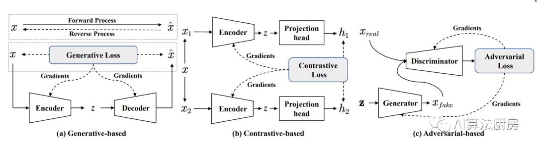
Self-supervised learning (SSL) methods can generally be divided into three categories:

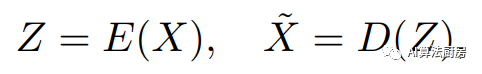
Generation-based methods: This method first uses an encoder to map the input x to a representation z, and then uses a decoder to reconstruct x from z. The training goal is to minimize the reconstruction error between the input and the reconstructed input. A common example of generative-based SSL is autoencoders, which learn efficient representations of input data by minimizing the error between the original input and the reconstructed input.
Contrast-based approach: This is one of the most widely used SSL strategies, which constructs positive and negative samples through data augmentation or context sampling. The model is then trained by maximizing the mutual information between two positive samples. Contrastive methods usually use contrastive similarity measures, such as InfoNCE loss. A well-known example of a contrast-based method is SimCLR, which learns effective image representations by comparing the representations of original and enhanced images.
Adversarial-based methods: This method usually consists of a generator and a discriminator. The generator generates fake samples, and the discriminator is used to distinguish them from real samples. A typical application of this approach is Generative Adversarial Networks (GANs), which find a balance between the generator and the discriminator through an adversarial process to generate realistic fake samples and improve the performance of the generator.

generation-based approach

In the context of time series modeling, commonly used preset tasks include using past sequences to predict future windows or specific timestamps, using encoders and decoders to reconstruct inputs, and predicting the invisibility of obscured time series part.

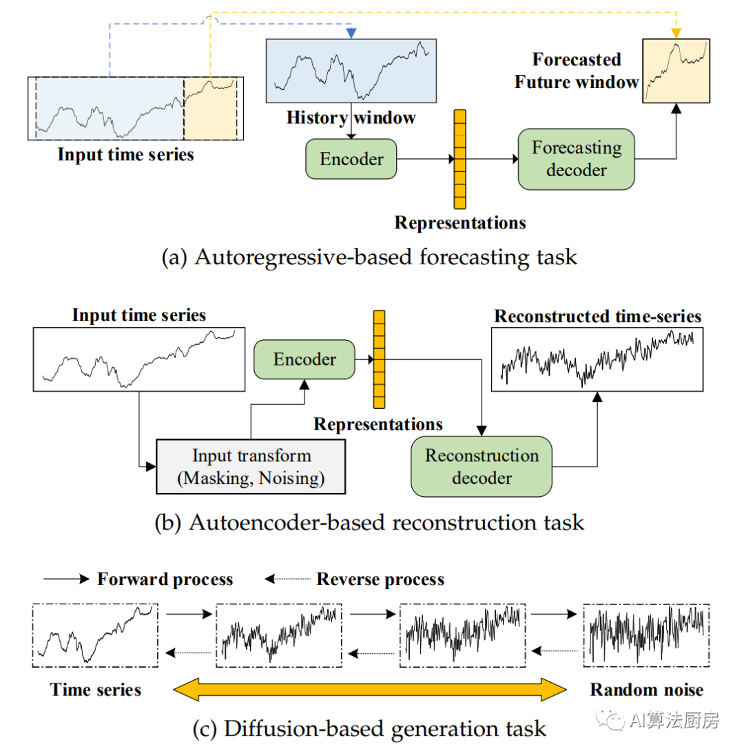
Forecasting based on autoregression

This method attempts to use past sequences (e.g., previous values of a time series) to predict future values.

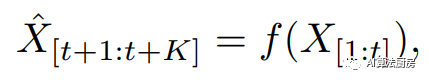
Among them is single-step prediction, and if it is greater than 1, it is multi-step prediction, which is the prediction function; the learning loss function hopes that the predicted future value will be as close as possible to the true value.

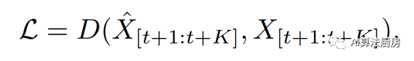
Among them is a description of distance, such as MSE.

Related work: THOC builds a self-supervised preset task for multi-resolution single-step prediction called Temporal Self-Supervision (TSS). TSS uses an L-layer expanded RNN with a skip connection structure as the model. By setting the jump length, you can ensure that the prediction task can be performed simultaneously at different resolutions. STraTS first encodes time series data into a ternary representation to avoid the limitations of using basic RNN and CNN when modeling irregular and sparse time series data, and then builds a Transformer-based predictive model for modeling multivariate medical clinical time sequence. Graph-based time series forecasting methods can also be used as self-supervised preset tasks. Compared with RNN and CNN, graph neural networks (GNNs) can better capture the correlation between variables in multivariate time series data, such as GDN. Different from the above methods, SSTSC proposes a temporal relationship learning prediction task based on the "past-anchor-future" strategy as a self-supervised preset task. SSTSC does not directly predict the value of the future time window, but predicts the relationship between time windows, which can fully mine the temporal relationship structure in the data.

Reconstruction based on autoencoders

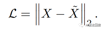
An autoencoder is an unsupervised artificial neural network composed of an encoder and a decoder. The encoder maps the input to a representation, and the decoder remaps the representation back to the input. The output of the decoder is defined as the reconstructed input.

where and represent the encoder and decoder respectively, which can be any form of neural network. The learned loss function is to hope that the reconstruction error is as small as possible.

Related work: TimeNet, PT-LSTM-SAE, and Autowarp all use RNN to build a sequence autoencoder model that includes an encoder and a decoder, and the model attempts to reconstruct the input sequence. Once the model is learned, the encoder is used as a feature extractor to obtain embedded representations of time series samples, which can help downstream tasks such as classification and prediction achieve better performance.

However, the representation obtained through the reconstruction error is task-independent. Therefore, introducing additional training constraints can be considered. Abdulaal et al. focused on complex asynchronous multivariate time series data and introduced spectral analysis in the autoencoder model. By learning the phase information in the data, a synchronized representation of the time series is extracted, which is ultimately used for anomaly detection tasks. DTCR is a representation learning model friendly to temporal clustering. It introduces K-means constraints in the reconstruction task, making the learned representation more friendly to the clustering task. USAD uses one encoder and two decoders to build an autoencoder model, and introduces adversarial training to enhance the model's representation capabilities. FuSAGNet introduces graph learning on sparse autoencoders to explicitly model relationships in multivariate time series.

Generation based on diffusion model

As a new type of deep generative model, diffusion models have recently achieved great success in many fields, including image synthesis, video generation, speech generation, bioinformatics, and natural language processing, due to their powerful generative capabilities. .

The key design of the diffusion model involves two opposing processes: a forward process that corrupts the data by injecting random noise, and a reverse process that generates samples from a noise distribution (usually a normal distribution). There are currently three basic forms of diffusion models: denoising diffusion probability models (DDPMs), fractional matching diffusion models, and fractional SDEs.

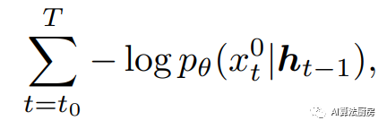
Related work: Conditional Fractional Diffusion Model for Interpolation (CSDI) proposes a new time series interpolation method that utilizes a fractional diffusion model based on observational data. It is trained for interpolation and can easily make predictions by inserting data at the end of a time series sequence. To deal with the problem of inaccessible real missing values in practice, a self-supervised training process is also proposed, in which values are marked as missing to train the entire architecture. In addition, there are several works utilizing diffusion models to predict time series. TimeGrad uses a conditional diffusion probability model at a certain time step to describe the fixed forward process and the learned reverse process. During the processing stage, time series cross-correlations are also plotted. It is an autoregressive model for multivariate time series forecasting that learns gradients by optimizing parameters that minimize the negative log-likelihood of the model.

comparison-based approach

Contrastive learning is a widely used self-supervised learning strategy that exhibits powerful learning capabilities in computer vision and natural language processing. Unlike discriminative models, which learn mapping rules to real labels, and generative models, which try to reconstruct the input, contrast-based methods aim to learn data representation through the comparison of positive and negative samples. Specifically, positive samples should have similar representations, while negative samples should have different representations. Therefore, the selection of positive and negative samples is very important for contrast-based methods.

Sampling comparison method

The sampling comparison method follows the widely used assumption in time series analysis that two adjacent time windows or timestamps have a high degree of similarity, and therefore, positive and negative samples are sampled directly from the original time series. Specifically, given a time window (or timestamp) as an anchor, windows (or timestamps) near it are more likely to be similar (small distance), while windows (or timestamps) far away should be less similar (distance big). "Similar" means that the two windows (or two timestamps) have more common patterns, such as the same amplitude, the same periodicity, and the same trend.

Forecast comparison method

In this category, the prediction task of using context (present information) to predict a target (future information) is considered a self-supervised pre-text task, where the goal is to maximize the mutual information of context and target. Contrastive Predictive Coding (CPC) provides a contrastive learning framework that uses InfoNCE loss to perform prediction tasks. Specifically, contexts and samples form positive pairs, while samples in the "proposal" distribution are negative samples. The learned loss function is

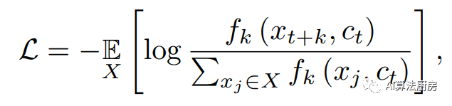
CPC does not directly predict future observations, but instead attempts to preserve the mutual information of sums. This enables the model to capture "slow features" that span multiple time steps. Based on the structure of CPC, LNT, TRL-CPC, TS-CP2 and Skip-Step CPC are proposed. LNT and TRL-CPC use the same structure as the original CPC to build a representation learning model, aiming to detect outliers by capturing the local semantics of time. TS-CP2 and Skip-Step CPC replace the autoregressive model in the original CPC structure with TCN, which improves feature learning capabilities and computational efficiency. In addition, Skip-Step CPC points out that adjusting the context representation and the distance between them can construct different positive sample pairs, which will lead to different results in time series anomaly detection. CMLF converts time series into coarse-grained and fine-grained representations and proposes a multi-granularity forecasting task. This enables the model to represent time series at different scales.

enhanced contrast method

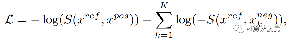
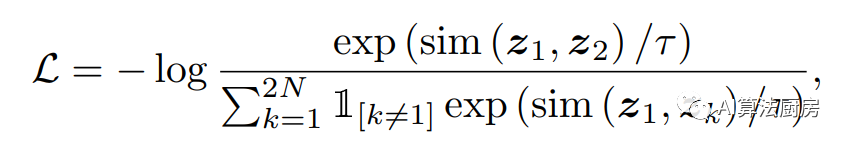
The enhanced contrast method is one of the most widely used contrast frameworks. Most methods utilize data augmentation techniques to generate different views of input samples and then learn representations by maximizing the similarity of views from the same sample and minimizing the similarity of views from different samples. SimCLR is a very typical representation learning framework based on multi-view invariance and has been adopted by many subsequent methods. The loss function under this framework is usually

Time series enhancement methods need to consider both time and variable dependencies, which is different from image enhancement methods.

Since time series data can be converted into frequency domain representation via Fourier transform, enhancement methods can be developed in both time and frequency domains. In the time domain, TS-TCC and its extended version CA-TCC design two time series data enhancement technologies - strong enhancement (Permutation-and-Jitter) and weak enhancement (Jitter-and-Scale). Another method, TS2Vec, generates different views by randomly masking certain time steps. In general, there is no unified standard answer to which data augmentation method to choose.

Data augmentation in the frequency domain is also feasible for time series data. There is a seasonal trend representation learning method called CoST, which uses fast Fourier transform to convert different enhanced views into amplitude and phase representations, and then trains these views through a specific training model. Another method, BTSF, is a contrastive method based on time-frequency fusion strategy. BTSF first generates an enhanced view in the time domain through a dropout operation, and then generates another enhanced view in the frequency domain through Fourier transform. Finally, the bilinear time-frequency fusion mechanism is used to achieve the fusion of time-frequency information. However, CoST and BTSF do not directly modify the frequency representation. In contrast, TF-C is the first work to enhance time series data through frequency perturbation, and its performance exceeds TS2Vec and TS-TCC. TF-C implements three enhancement strategies: low-frequency to high-frequency perturbation, single-component to multi-component perturbation, and random to distributed perturbation.

Prototype comparison method

The prototype contrastive learning framework is essentially an instance discrimination task, which encourages samples to form a uniform distribution in the feature space. However, the real data distribution should satisfy that similar samples are more concentrated in one cluster, while the distance between different clusters should be farther. SCL is an ideal solution when real labels are available, but in practice, especially with time series data, this is difficult to implement. Therefore, introducing clustering constraints into existing contrastive learning frameworks is an alternative, such as CC, PCL, and SwAV. PCL and SwAV compare samples with constructed prototypes, i.e., cluster centers, which reduces the computational effort and encourages samples to present a cluster-friendly distribution in the feature space.

In prototype contrast-based time series modeling, ShapeNet takes Shaplets as input and constructs a cluster-level triplet loss that considers the distance between the anchor point and multiple positive (negative) samples, as well as the positive (Negative) distance between samples. ShapeNet is an implicit prototype comparison because it does not introduce explicit prototypes (clustering centers) during the training phase. TapNet and VSML are explicit prototype comparisons because they introduce explicit prototypes. TapNet introduces a learnable prototype for each predefined category and performs classification based on the distance between the input time series samples and each category prototype. VSML defines virtual sequences that perform the same function as prototypes, i.e., minimize the distance between samples and virtual sequences, but maximize the distance between virtual sequences.

MHCCL proposes a hierarchical clustering based on the upward masking strategy and a comparison selection strategy based on the downward masking strategy. In the upward masking strategy, MHCCL considers outliers to have a great impact on the prototype, so these outliers should be removed when updating the prototype. In turn, the downward masking strategy uses the clustering results to select positive and negative samples, i.e., samples belonging to the same prototype are considered true positive samples, while samples belonging to different prototypes are considered true negative samples.

expert knowledge comparison method

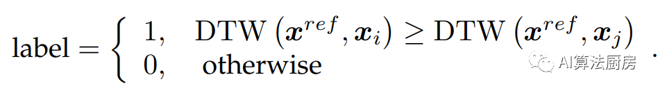
Expert knowledge comparison is a relatively new framework for representation learning. Generally speaking, this modeling framework incorporates experts’ prior knowledge or information into deep neural networks to guide model training. In the contrastive learning framework, prior knowledge can help the model select the correct positive and negative samples during the training process.

For example, Shi et al. used the DTW distance of time series samples as prior information, and believed that two samples with a small distance have higher similarity. Specifically, given an anchor point and two other samples, the DTW distance between the anchor point and the other two samples is first calculated, and then the sample with a small distance from the anchor point is regarded as a positive sample of the anchor point.

adversarial approach

Adversarial-based self-supervised representation learning methods use generative adversarial networks (GANs) to build pre-text tasks. GAN contains a generator G and a discriminator D. The generator G is responsible for generating synthetic data similar to real data, while the discriminator D is responsible for determining whether the generated data is real data or synthetic data. Therefore, the goal of the generator is to maximize the decision failure rate of the discriminator, and the goal of the discriminator is to minimize its failure rate. The generator G and the discriminator D are in a game relationship with each other.

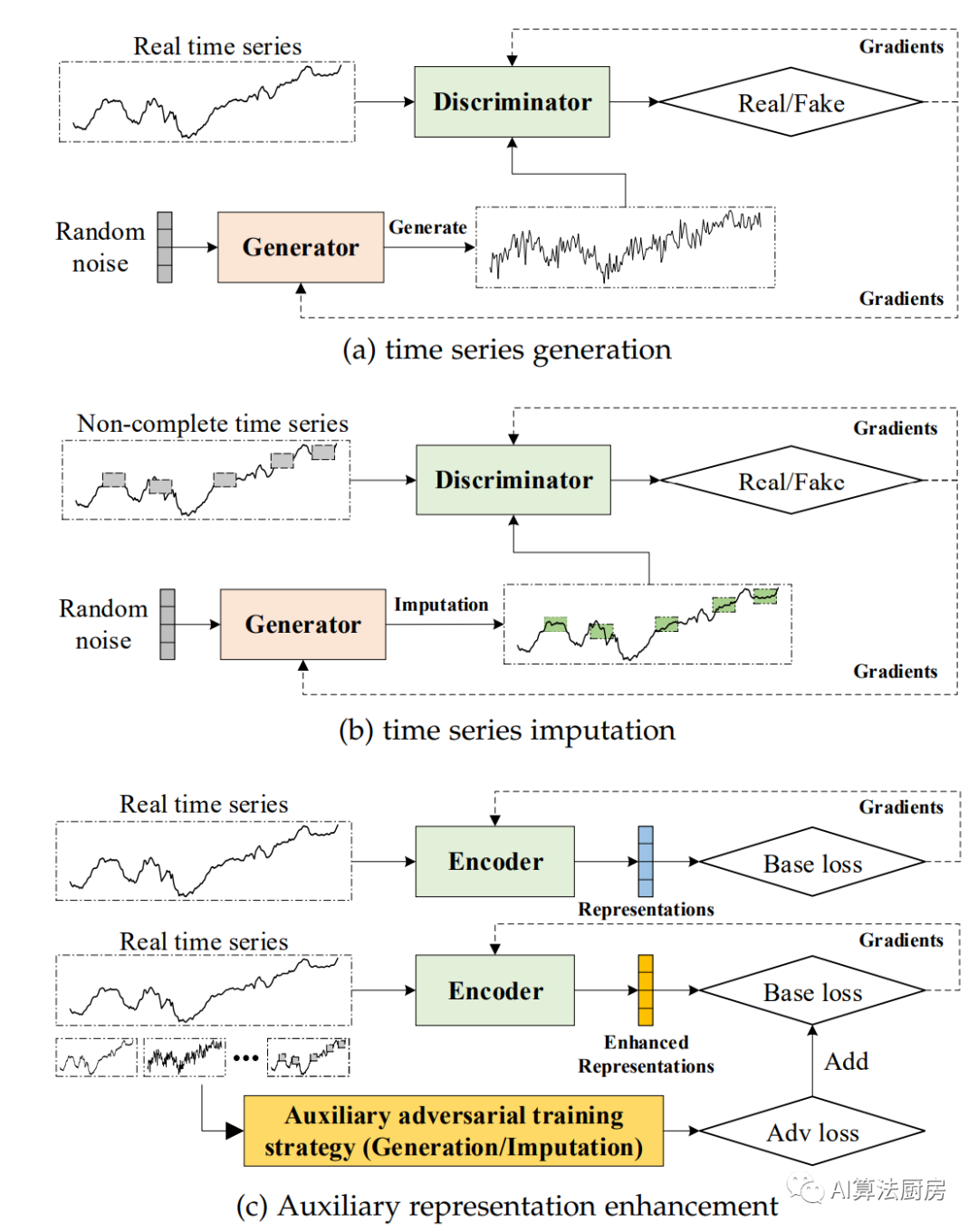
Time series generation and imputation

Complete time series generation refers to generating a new non-existing time series in an existing data set. New samples can be univariate or multivariate time series. C-RNN-GAN is an early method of using GAN to generate time series samples. The generator is an RNN and the discriminator is a bidirectional RNN. RNN-based structures can capture the dynamic dependencies of multiple time steps but ignore the static characteristics of the data. TimeGAN is an improved time series generation framework that combines basic GAN with autoregressive models, allowing the temporal dynamic characteristics of the series to be preserved. TimeGAN also emphasizes that static features and temporal features are crucial for generation tasks.

Some recently proposed methods consider more complex time series generation tasks. For example, COSCI-GAN is a time series generation framework that considers the relationship between each dimension in a multivariate time series. It includes Channel GANs and Central Discriminator. Channel GANs are responsible for independently generating data for each dimension, while Central Discriminator is responsible for determining whether the relationship between different dimensions of the generated sequence is the same as the original sequence. PSA-GAN is a framework for long-term sequence generation and introduces a self-attention mechanism. TTS-GAN explores the generation of time series data with irregular spatiotemporal relationships. This method uses Transformer to build the discriminator and generator, and treats the time series data as image data with a height of one.

Different from generating new time series, the task of time series imputation is given an incomplete time series sample (e.g., data for some time steps is missing), and the missing values need to be filled based on contextual information. Luo et al. treat the problem of missing value imputation as a data generation task and use a generative adversarial network (GAN) to learn the distribution of the training data set. In order to better capture the dynamic characteristics of the series, they proposed the GRUI module. The GRUI module uses a time lag matrix to record the time lag information between effective values of incomplete time series data. This information follows an unknown non-uniform distribution and is very helpful for analyzing the dynamic characteristics of the sequence. The GRUI module is further used in E2GAN. SSGAN is a semi-supervised framework for time series data interpolation, which includes a generative network, a discriminative network and a classification network. Unlike previous frameworks, SSGAN's classification network fully utilizes label information, which helps the model achieve more accurate interpolation.

Auxiliary representation enhancement

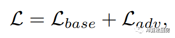
In addition to generation and interpolation tasks, adversarial-based representation learning strategies can be added to existing learning frameworks as additional auxiliary learning modules, which we refer to as adversarial-based auxiliary representation enhancement. Auxiliary representation enhancement aims to promote the model to learn more informative representations for downstream tasks by adding adversarial-based learning strategies. Usually defined as follows

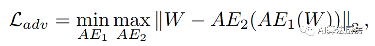
USAD is a time series anomaly detection framework that includes two BAE models, which are defined as AE1 and AE2 respectively. The core idea behind USAD is to amplify the reconstruction error through adversarial training between two BAEs. In USAD, AE1 is regarded as the generator and AE2 is regarded as the discriminator. The auxiliary goal is to use AE2 to distinguish AE1's reconstructed data from real data, and train AE1 to deceive AE2.

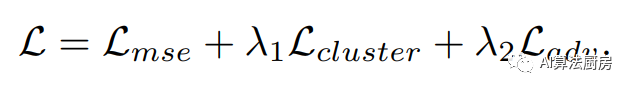
DUBCNs and CRLI are used for series retrieval and clustering tasks respectively. Both methods adopt RNN-based BAE as the model and add clustering-based loss and adversarial-based loss to the basic reconstruction loss.

Application selection

Self-supervised learning (SSL) has wide applications in various time series tasks, such as prediction, classification, anomaly detection, etc.

abnormal detection

The problem of anomaly detection in time series is mainly to identify abnormal time points or abnormal time series based on certain specifications or common signals. Since obtaining labels for abnormal data is challenging, most time series anomaly detection methods employ unsupervised learning frameworks. Among them, autoregression-based prediction and autoencoder-based reconstruction are the most commonly used modeling strategies. For example, THOC and GDN use a self-supervised learning framework for autoregressive prediction, which assumes that abnormal sequences or time points are unpredictable. RANSynCoders, USAD, AnomalyTrans and DAEMON use a self-supervised learning framework based on autoencoder reconstruction. The principle of this framework is that abnormal data is difficult to reconstruct. Furthermore, VGCRN and FuSAGNet combine the two frameworks to achieve more robust and accurate detection results. Introducing adversarial-based self-supervised learning methods in detection models can further expand the difference between normal data and abnormal data, such as USAD and DAEMON.

predict

Time series forecasting is the prediction of future time windows or points in time by using statistical and modeling techniques to analyze time series data. The pre-text task based on autoregressive prediction is essentially a time series prediction task. Therefore, various models based on prediction tasks have been proposed, such as Pyraformer, FilM, Quatformer, Informer, Triformer, Scaleformer, Crossformer, and Timesnet. We found that decomposing time series (such as seasonality and trend) and then learning and forecasting on the decomposed components can improve the accuracy of the final forecast, such as MICN and CoST. When there are missing values in the time series, it is feasible to introduce adversarial self-supervised learning. For example, LGnet introduces adversarial training to enhance the modeling of global temporal distribution, which reduces the impact of missing values on prediction accuracy.

Classification and clustering

The goal of classification and clustering tasks is to identify the true class to which a specific time series sample belongs. Since the core of contrastive learning is to identify positive and negative samples, contrast-based self-supervised learning methods are the best choice for these two tasks. Specifically, TSTCC introduces temporal contrast and contextual contrast to obtain a more robust representation. TS2Vec and MHCCL perform hierarchical contrastive learning strategies on enhanced views, which makes it possible to obtain more robust representations. Similar to anomaly detection and prediction tasks, adversarial-based self-supervised learning strategies can also be introduced into classification and clustering tasks. For example, DTCR proposes a fake sample generation strategy to help the encoder obtain a more expressive representation.

In summary, generation-based self-supervised learning is more suitable for anomaly detection and prediction tasks, while contrast-based self-supervised learning is more suitable for classification and clustering tasks. Adversarial-based self-supervised learning can play a role in a variety of tasks, but in most cases it is used as an additional regularization term to ensure that the features extracted by the model are more robust and informative.

references

Self-Supervised Learning for Time Series Analysis: Taxonomy, Progress, and Prospects

A review and interpretation of self-supervised learning for time series

Guess you like