How to attack neural networks? Artificial Intelligence VS Artificial Mental Retardation

I. Introduction

Since 2012, artificial intelligence has developed rapidly and frequently appears in the public eye. From Alpha GO to ChatGPT, artificial intelligence has become an unstoppable development trend. However, due to the black-box nature of neural learning, neural networks are difficult to explain and difficult to control. Even a powerful model like ChatGPT will have some low-level errors when connected to the Internet.

Neural network errors are hard to figure out. For example, face detection sometimes detects faces that have nothing to do with faces (to humans). ChatGPT will also answer some clueless answers. For example, when GPT3.5 encounters the problem "2022 Van der Sar points occur", a short circuit will occur. Or Lee Sedol's "God's Hand", which are all elusive manifestations of neural networks.

Today’s topic is not about why these situations occur, but how to create them, that is, attack neural networks. After reading today’s content, I believe everyone will have a new understanding of the intelligence of neural networks.

2. Online training

Now no matter what network it is, almost all gradient descent algorithms are used. First, you need to define a network, which is represented here by y=f(θ;x), where θ is the weight of the network. There are infinite possibilities for the optional value of θ, but only a few θ can get better results. In order to evaluate the quality of θ, a loss function loss=L(f(θ;x), target) can be defined, where target is the real value. Now you only need to find a set of θ that minimizes the loss to complete the training.

However, f(θ;x) is a very complex function, and L(f(θ;x), target) is even more complicated and cannot directly give an analytical solution, so iterative algorithm needs to be used to solve θ. The gradient descent algorithm is used in deep learning. The expression of the gradient descent algorithm is as follows:

$$i=i-the\frac{\partial L}{\partial \theta }$$

Among them, eta is a parameter used to adjust the update amplitude, called the learning rate. When the loss is relatively small, the network can predict the results correctly. The attacks also revolve around gradient and loss. Attacking the network is to generate an adversarial sample so that a larger loss can be obtained after inputting this sample into the network. Or let the adversarial sample have a small loss with the false true value.

3. Adversarial Attack

黑盒攻击There are many ways to attack neural networks, which can be divided into sums based on different prior knowledge 白盒攻击. Based on different purposes, it can be divided into 源/目标误分类, 针对性误分类, 误分类, and 置信度降低. Among them 误分类, the simplest purpose of the attack is to make the model classify incorrectly. This is also an attack to be implemented in this article.

Among them, white-box attack is relatively simple. In white-box attack, we know the model well. We know every detail of the network, and we can also get the network for inference and gradient backpropagation. In white-box attacks, adversarial examples can be generated through gradient information. During the training process, our goal is to reduce the loss, while the confrontation process is to increase the loss. When the generated adversarial sample calculates a larger loss, the network will have a greater probability of classification error, thus achieving the purpose of deceiving the network.

Black box attacks are more complex. Black box attacks assume that we do not know the detailed information of the network, network structure, and network weights, but we can use this network. We know what the input to the network is and what the output corresponds to the current input. In this case, attacking the neural network will be more complicated.

Networks that have gone online are usually in a black box situation. After the adversarial samples are proposed, everyone does not think that the network can be attacked correctly in a black box situation. Goodfellow, the author of GAN, found that this is not the case. Black box attacks can be implemented using integrated learning, which will not be introduced in detail in this article. This article mainly discusses white box attacks.

四、Fast Gradient Sign Attack

There are also various ways to implement attacks. This article uses an Fast Gradient Sign Attack(FGSA)attack method called , which uses gradient information to modify the input to achieve the purpose of the attack.

As mentioned earlier, model training is implemented using the gradient descent algorithm. There are two points to note here, one is the update direction and the other is the update parameters. During the training process, our goal is to minimize L(f(θ;x), target) and find an optimal set of θ. From this we can know that the parameter we want to update is θ, and the update direction is the opposite direction of the gradient.

The purpose of the attack model is different. First, the case of misclassification is discussed. In the case of misclassification, our goal is to generate adversarial samples to make the model misclassify. At this time, our goal is to make L(f(θ;x), target) relatively large. What we are looking for here is an adversarial example, so the updated parameter is x, and the direction is the gradient direction. Then the operation of generating adversarial samples can be expressed by the following formula:

$$adversarialX=x+ϵ\frac{\partial L}{\partial x}$$

In FGSA, the gradient size is not considered, only the gradient direction is concerned. Therefore, the following formula should be used in FGSA:

$$adversarialX=x+ϵsign(\frac{\partial L}{\partial x})$$

where sign is the sign function, which returns the sign of the gradient.

4. Code implementation

Next, we use the code to implement the FGSA attack, here we use a white box attack. So we need to implement a network first, here we take handwritten numbers as an example.

4.1 Handwritten digit recognition

The characteristic of a white-box attack is that we know all the details of the network, so we implement a network ourselves, and we can know all the details of this network. The network can be freely designed. Here we choose to use a two-layer convolutional neural network. The training code is as follows:

import torch
from torch import nn
from torch import optim
from torch.utils.data import DataLoader
from torchvision import datasets
from torchvision.transforms import ToTensor
from collections import OrderedDict

device = "cuda" if torch.cuda.is_available() else "cpu"

# 超参数
epochs = 10
batch_size = 64
lr = 0.001

# 1、加载数据
train_dataset = datasets.MNIST('./', True, ToTensor(), download=True)
train_loader = DataLoader(train_dataset, batch_size)


# 2、构建模型
class DigitalNet(nn.Module):
    def __init__(self):
        super(DigitalNet, self).__init__()
        self.model = nn.Sequential(OrderedDict({
            "conv1": nn.Conv2d(1, 6, 5),
            "relu1": nn.ReLU(),
            "pool1": nn.MaxPool2d(2),
            "conv2": nn.Conv2d(6, 16, 5),
            "relu2": nn.ReLU(),
            "pool2": nn.MaxPool2d(2),
            "flatten": nn.Flatten(),
            "fc1": nn.Linear(4 * 4 * 16, 128),
            "relu3": nn.ReLU(),
            "fc2": nn.Linear(128, 10),
        }))

    def forward(self, inputs):
        return self.model(inputs)


# 3、定义loss
loss_fn = nn.CrossEntropyLoss()
# 4、定义优化器
model = DigitalNet().to(device)
optimizer = optim.Adam(model.parameters(), lr)
# 5、训练
for epoch in range(epochs):
    for image, target in train_loader:
        image, target = image.to(device), target.to(device)
        # 正向传播
        output = model(image)
        loss = loss_fn(output, target)
        model.zero_grad()
        # 反向传播
        loss.backward()
        # 更新参数
        optimizer.step()
    print(f'epoch: {epoch+1}, loss: {loss.item()}')
    torch.save(model.state_dict(), 'digital.pth')

For convenience, the test-related code is omitted here, and the calculation of the accuracy rate is also omitted. After the code runs, you can get a digital.pthfile, which is the model file. This file is needed for subsequent generation of adversarial examples.

4.2 FGSA

Once we have the model, we can start generating adversarial examples. The FGSA method is used here. In the previous we derived the expression of FGSA as:

$$adversarialX=x+ϵsign(\frac{\partial L}{\partial x})$$

Now you only need to implement this function with code. This function has two inputs, namely the input x and the gradient of x. The operation of this function can be divided into the following steps:

1. Get gradient direction
2. Substitute into the above formula to get the adversarial sample

code show as below:

def fgsa_attack(x, epsilon, x_grad):
    # 获取x梯度方向
    sign_grad = x_grad.sign()
    # 更新x，让x往梯度方向更新
    adversarial_x = x + epsilon * sign_grad
    # 把结果映射到0-1之间
    adversarial_x = torch.clamp(adversarial_x, 0, 1)
    return adversarial_x

Among them, x is our existing data, epsilon is a hyperparameter, which needs to be set by ourselves, and x_grad is the gradient information of x, which has not been obtained yet. The next thing to do is to get x_grad, which is to find the derivative of the loss function with respect to x.

By default, x will not be derived, so you need to set x to be automatically derived, just need the following sentence:

x.requires_grad = True

The next thing to do is to calculate the loss and backpropagate it. After calling the loss.backward() method, the gradient information is stored in the tensor, and the gradient of x can be obtained in the following way:

x_grad = x.grad.data

In this way, we have all the values ​​required by fgsa_attack, and then we can generate adversarial samples. The complete code to attack the network is as follows:

import torch
from torch import nn
from torch.utils.data import DataLoader
from torchvision import datasets, utils
from torchvision.transforms import ToTensor
from collections import OrderedDict
import matplotlib.pyplot as plt

device = "cuda" if torch.cuda.is_available() else "cpu"

# 超参数
epochs = 10
batch_size = 64
lr = 0.001

# 1、加载数据
train_dataset = datasets.MNIST('./', True, ToTensor(), download=True)
train_loader = DataLoader(train_dataset, batch_size)


loss_fn = nn.CrossEntropyLoss()
# 加载模型
model = DigitalNet()
model.load_state_dict(torch.load('digital.pth'))
for image, target in train_loader:
    # 设置输入自动求导
    image.requires_grad = True
    output = model(image)
    loss = loss_fn(output, target)
    model.zero_grad()
    loss.backward()
    # loss对image的梯度
    image_grad = image.grad.data
    # 对image进行修改
    adversarial_x = fgsa_attack(image, .15, image_grad)
    # 对攻击数据预测
    output = model(adversarial_x)
    grid = utils.make_grid(adversarial_x, normalize=True)
    with torch.no_grad():
        grid = grid.cpu().numpy().transpose((1, 2, 0))
        print(output.argmax(dim=1).cpu().numpy().reshape((8, 8)))
        plt.imshow(grid)
        plt.show()
    break

64 images were tested here, and the following is the offensive input image:

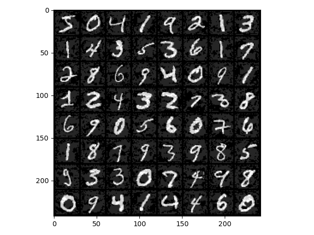
For people, this image is still the original number, but for the neural network, this is not the case. The following matrix is ​​the prediction result corresponding to each image:

[[2 9 3 8 8 9 8 8]
 [3 3 0 8 8 8 8 8]
 [8 7 3 2 9 5 8 8]
 [3 3 8 3 7 2 7 7]
 [9 7 0 2 3 0 2 9]
 [8 3 5 8 8 8 8 8]
 [5 0 5 0 5 3 8 7]
 [5 8 9 8 2 7 3 5]]

4.3 Classify into specified categories

In the previous program, we only asked to generate data and let the network misclassify it. In some scenarios, we need to generate data for the network to classify into specified categories. For example, if we want to fool face recognition, we need to generate data that allows the network to identify someone. How should this be achieved? In fact, it is very simple. The operation of misclassification is to change the input and update the gradient direction of the input network. At this time, the loss will increase, thereby achieving the effect of misclassification.

Misclassification into a certain category is different. For example, if we now want to generate data so that the model misclassifies it into the number 1, what we need to do is to make it loss_fn(output, 1)smaller, so we need to modify two places:

1. Target value changed to 1 (category specific)
2. Data is updated in the opposite direction of the gradient

Now modify the fgsa_attack function as follows:

def fgsm_attack(x, epsilon, x_grad):
    # 获取梯度的反方向
    sign_grad = -x_grad.sign()
    # 让输入添加梯度信息，即让输入添加能让loss减小的信息
    adversarial_x = x + epsilon * sign_grad
    # 把结果映射到0-1之间
    adversarial_x = torch.clamp(adversarial_x, 0, 1)
    return adversarial_x

Modify the attack code to:

import torch
from torch import nn
from torch.utils.data import DataLoader
from torchvision import datasets, utils
from torchvision.transforms import ToTensor
from collections import OrderedDict
import matplotlib.pyplot as plt

device = "cuda" if torch.cuda.is_available() else "cpu"

# 超参数
epochs = 10
batch_size = 64
lr = 0.001

# 1、加载数据
train_dataset = datasets.MNIST('./', True, ToTensor(), download=True)
train_loader = DataLoader(train_dataset, batch_size)


loss_fn = nn.CrossEntropyLoss()
# 加载模型
model = DigitalNet()
model.load_state_dict(torch.load('digital.pth'))
for image, target in train_loader:
    # 设置输入自动求导
    image.requires_grad = True
    output = model(image)
    # 把目标值修改为1
    target[::] = 1
    loss = loss_fn(output, target)
    model.zero_grad()
    loss.backward()
    # loss对image的梯度
    image_grad = image.grad.data
    # 对image进行修改
    adversarial_x = fgsa_attack(image, .2, image_grad)
    # 对攻击数据预测
    output = model(adversarial_x)
    grid = utils.make_grid(adversarial_x, normalize=True)
    with torch.no_grad():
        grid = grid.cpu().numpy().transpose((1, 2, 0))
        print(output.argmax(dim=1).cpu().numpy().reshape((8, 8)))
        plt.imshow(grid)
        plt.show()
    break

What is done here is to change the target value to 1 and adjust the epsilon value of fgsa_attack. The resulting attack image is as follows:

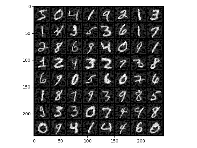
The model's prediction result for the image is:

[[3 0 1 1 4 8 1 1]
 [1 1 1 1 3 6 1 9]
 [0 1 1 1 1 1 1 1]
 [1 1 8 1 0 1 1 1]
 [5 1 1 1 1 0 1 1]
 [1 1 1 1 3 4 8 1]
 [1 1 1 9 0 8 4 1]
 [0 4 1 1 9 1 5 9]]

Although the results are not all 1, the number of predicted 1 results is far more than the actual number of 1, indicating that the attack is successful.

5. Summary

Neural networks are very powerful, but their understanding is still an open problem. Because the neural network is very large, it is difficult for us to grasp every detail and determine how the network infers the results. Because of this, a seemingly well-trained model will have many bizarre phenomena when applied to actual tasks. Only by understanding why these strange phenomena occur can we better understand the model and improve the model.

Because most networks today use gradient descent to update the model, gradients are a good breaking point for attacking the network. Two attacks were performed on the network above, both seemingly very effective. However, the premise of a white-box attack is that we can know the specific structure of the network and have complete control over the network. However, in actual situations, this is not common, so there is no need to worry too much about your network being attacked.