A small practice that I had time to tinker with on weekends was mainly for the task of multi-factor regression prediction. I have introduced it in detail in my columns and series of blog posts about time series data modeling and regression prediction modeling. Here is the introduction. I won’t go into details anymore. This is mainly a practice of model fusion. The data here is a domain data set generated by simulation. It is a typical tabular data set. First, let’s look at the data sample:
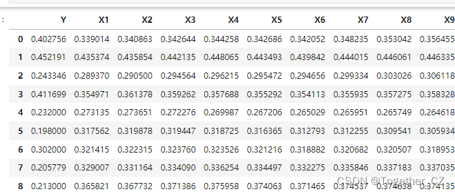
The basic data processing implementation is as shown:
import pandas as pd

# 读取 "data" 工作表的内容
sheet_name = "data"
data = pd.read_excel("dataset.xlsx", sheet_name=sheet_name)

# 删除第一列日期列
data1= data.iloc[:, 1:]

print(data1.head(20))
Next, the data set is randomly divided, and the implementation is as follows:
from sklearn.model_selection import train_test_split
X = data.drop(columns=['Y'])  # 这将删除名为'label'的列,并返回其余部分
y = data['Y']
x_train, x_test, y_train, y_test = train_test_split(X, y, test_size=0.2, random_state=42)
Next, the data is normalized and calculated as follows:
# 创建特征标准化的对象
scaler = StandardScaler()  # 或者使用 MinMaxScaler() 来进行 Min-Max 缩放

# 训练标准化对象并转换训练特征
x_train_scaled = scaler.fit_transform(x_train)

# 假设你有测试数据 x_test 和 y_test,对测试特征进行相同的变换
x_test_scaled = scaler.transform(x_test)

# 输出尺寸
print("训练特征(标准化后)的尺寸:", x_train_scaled.shape)
print("测试特征(标准化后)的尺寸:", x_test_scaled.shape)
print("特征列(x_train)的尺寸:", x_train.shape)
print("标签列(y_train)的尺寸:", y_train.shape)
print("特征列(x_test)的尺寸:", x_test.shape)
print("标签列(y_test)的尺寸:", y_test.shape)
Next is the data conversion process:
def reshape_to_window(data, window=window):
    """
    数据转化
    """
    n = data.shape[0]
    m = data.shape[1]
    result = np.zeros((n - window + 1, window, m))
    for i in range(n - window + 1):
        result[i] = data[i:i+window]
    return result


x_train = reshape_to_window(x_train, window)
y_train = y_train.iloc[window-1:]

x_test = reshape_to_window(x_test, window)
y_test = y_test.iloc[window-1:]

print("新的x_train形状:", x_train .shape )
print("新的y_train形状:", y_train .shape)
print("新的x_test形状:", x_test.shape)
print("新的y_test形状:", y_test.shape)
Next, the model is initialized and built based on the keras framework. The model part here mainly uses DCNN and LSTM to fuse them. First, let’s look at the overall regression of DCNN and LSTM:
DCNN
Dilated convolution (dilated convolution) is a convolution operation in Convolutional Neural Network (CNN). It expands the receptive field (receptive field) by adding holes (dilation) to the convolution kernel, thereby improving Model robustness and generalization ability.
In traditional convolution operations, the convolution kernel can only cover a small part of the feature map, but by adding holes to the convolution kernel, the convolution kernel can slide between adjacent feature maps, thus extending the convolution The receptive field of the core enhances the expressive ability of the model. The basic principle of atrous convolution is to set the sliding step of the traditional convolution operation to 1, and then divide the size of the convolution kernel (kernel size) by 2, so that the center point of the convolution kernel can be aligned with any point on the feature map. The convolution operation is performed on the pixels at the position.
In dilated convolution, each convolutional layer has a different number of dilation rates, which represents the number of holes added in each convolutional layer. The higher the hole rate, the larger the receptive field of the convolution kernel, and more feature information can be extracted. However, too high a hole rate will cause the feature map to become sparse, making it difficult to capture detailed information. Therefore, there is a trade-off between the hole rate and the sparsity of the feature map in atrous convolution.
Atrous convolution can be applied to multiple tasks in deep convolutional neural networks, such as image classification, target detection, semantic segmentation, etc. Compared with traditional convolution operations, dilated convolution can improve the robustness and generalization ability of the model, while reducing the amount of calculation and the number of parameters, making the model more lightweight and efficient.
LSTM
LSTM (Long Short-Term Memory) is a variant of Recurrent Neural Network (RNN) that is particularly suitable for processing sequence data. Compared with traditional RNN, LSTM has better performance and stability when processing time series data.
LSTM consists of forget gate, input gate, output gate and cell state. The forgetting gate determines which information in the memory state of the previous moment should be forgotten, the input gate determines which of the currently input information should be used to calculate the output, the output gate determines the output at the current moment, and the storage unit is used for storage and output the memory status at the current moment.
The core idea of LSTM is to control the flow of information through forget gates and input gates to achieve a balance between long-term dependence and short-term dependence. The forgetting gate and the input gate are both composed of sigmoid function and linear layer, while the output gate is composed of sigmoid function, linear layer and ReLU function. These gates control the flow direction and intensity of information, allowing LSTM to handle long-term dependencies.
In addition to LSTM, there are also recurrent neural network variants such as GRU (Gated Recurrent Unit) and SRU (Simple Recurrent Unit), which are similar to LSTM in structure and performance. LSTM is widely used in natural language processing, speech recognition, image processing and other fields.
The code implementation of the model part is as follows:
from tensorflow.keras import backend as K

# # 输入参数

input_size = 176  # 你的输入尺寸
lstm_units =16# 你的LSTM单元数
dropout = 0.01    # 你的dropout率

# 定义模型结构
inputs = Input(shape=(window, input_size))

# 第一层空洞卷积
model = Conv1D(filters=lstm_units, kernel_size=1, dilation_rate=1, activation='relu')(inputs)
# model = MaxPooling1D(pool_size=1)(model)
# model = Dropout(dropout)(model)

# 第二层空洞卷积
model = Conv1D(filters=lstm_units, kernel_size=1, dilation_rate=2, activation='relu')(model)
# model = MaxPooling1D(pool_size=1)(model)

# 第三层空洞卷积
model = Conv1D(filters=lstm_units, kernel_size=1, dilation_rate=4, activation='relu')(model)
# model = MaxPooling1D(pool_size=1)(model)
# model = BatchNormalization()(model)

# LSTM层
model = LSTM(lstm_units, return_sequences=False)(model)

# 输出层
outputs = Dense(1)(model)

# 创建和编译模型
model = Model(inputs=inputs, outputs=outputs)

model.compile(loss='mse', optimizer='adam', metrics=['mse'])
model.summary()
The summary output looks like this:
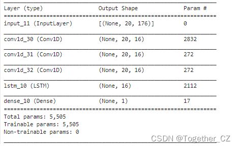
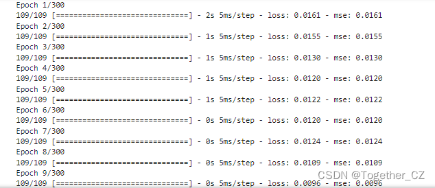
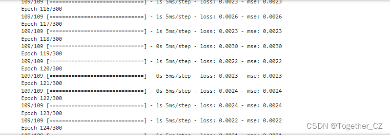
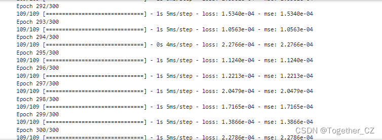
Next, you can start model training, and the log output is as follows:
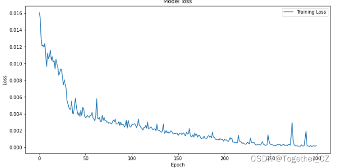
Next, visualize the loss during the overall training process of the model, as shown below:
plt.figure(figsize=(12, 6))
plt.plot(history.history['loss'], label='Training Loss')
plt.title('Model loss')
plt.ylabel('Loss')
plt.xlabel('Epoch')
plt.legend(loc='upper right')
plt.show()
The result looks like this:
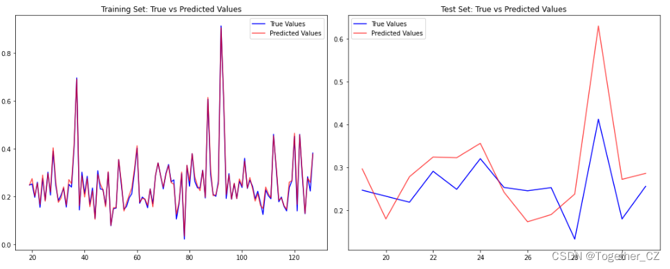
Next, conduct a comparative prediction analysis on the test set, as shown below:
explained_variance_score: explains the variance score of the regression model. Its value range is [0,1]. The closer it is to 1, the better the independent variable can explain the
variance change of the dependent variable. The smaller the value, the worse the effect.
mean_absolute_error: Mean Absolute Error (MAE), used to evaluate the closeness of the prediction results to the real data set
. The smaller the value, the better the fitting effect.
mean_squared_error: Mean squared error (MSE). This indicator calculates the mean of the sum of squares of the errors between the fitted data and the original data corresponding to the sample points. The smaller the value, the better the fitting effect
.
r2_score: coefficient of determination, which means the score that explains the variance of the regression model. Its value range is [0,1]. The closer it is to 1, the more the independent variable can explain the variance change of the dependent variable. The smaller the value, the better the effect
. The worse.
The model is evaluated and calculated based on the regression model evaluation indicators. The core code implementation is as follows:
#!usr/bin/env python
#encoding:utf-8
from __future__ import division


'''
__Author__:沂水寒城
功能:计算回归分析模型中常用的四大评价指标
'''

from sklearn.metrics import explained_variance_score, mean_absolute_error, mean_squared_error, r2_score


def calPerformance(y_true,y_pred):
    '''
    模型效果指标评估
    y_true:真实的数据值
    y_pred:回归模型预测的数据值
    '''
    model_metrics_name=[explained_variance_score, mean_absolute_error, mean_squared_error, r2_score]
    tmp_list=[]
    for one in model_metrics_name:
        tmp_score=one(y_true,y_pred)
        tmp_list.append(tmp_score)
    print ['explained_variance_score','mean_absolute_error','mean_squared_error','r2_score']
    print tmp_list
    return tmp_list


def mape(y_true, y_pred):
    return np.mean(np.abs((y_pred - y_true) / y_true)) * 100
from sklearn.metrics import r2_score
RMSE = mean_squared_error(y_train_predict, y_train)**0.5
print('训练集上的/RMSE/MAE/MSE/MAPE/R^2')
print(RMSE)
print(mean_absolute_error(y_train_predict, y_train))
print(mean_squared_error(y_train_predict, y_train) )
print(mape(y_train_predict, y_train) )
print(r2_score(y_train_predict, y_train) )


RMSE2 = mean_squared_error(y_test_predict, y_test)**0.5
print('测试集上的/RMSE/MAE/MSE/MAPE/R^2')
print(RMSE2)
print(mean_absolute_error(y_test_predict, y_test))
print(mean_squared_error(y_test_predict, y_test))
print(mape(y_test_predict,  y_test))
print(r2_score(y_test_predict, y_test))
The resulting output looks like this:
训练集上的/RMSE/MAE/MSE/MAPE/R^2
0.011460134959888058
0.00918032687965506
0.00013133469329884847
4.304916429848429
0.9907179432442654
测试集上的/RMSE/MAE/MSE/MAPE/R^2
0.08477191056357428
0.06885029105374023
0.007186276820598636
24.05688263657184
0.4264760739398442
If you are interested in content related to regression modeling, you can refer to my previous article:
"Summary Record of Commonly Used Data Regression Modeling Algorithms"