This chapter discusses the basic mechanisms for plotting function graphs and data graphs. Key examples are plotting functions of one variable, and displaying values read from a file.

15.1 Introduction

Our main goal is not the aesthetics of the output, but an understanding of how such graphical output is generated and the programming techniques used. You will find that the design techniques, programming techniques, and basic mathematical tools used in this chapter are of more lasting value than the graphical capabilities demonstrated.

15.2 Drawing simple function graphs

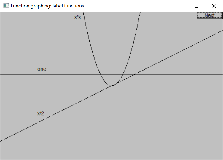
The code below plots $y = 1$ 、 $\frac{x}{2}$ y $x^2$ functions:

Draw a simple function graph

First a set of constants are defined to avoid "magic numbers", and then three are defined Function. Its first argument (with one argument, returning a function) draws in the Functionwindow , the second and third arguments specify the range (domain) of the argument, and the fourth argument specifies the location of the origin in the window, The last three parameters are explained in the next section.doubledouble

Note: FunctionThe y-axis is automatically flipped up and down.

The following uses Textan object to label a function image:

Text ts(Point(100, y_orig - 40), "one");
Text ts2(Point(100, y_orig + y_orig / 2 - 20), "x/2");
Text ts3(Point(x_orig - 100, 20), "x*x");

add tag

For more clarity, Axisadd axes using objects:

const int xlength = xmax - 40;  // make the axis a bit smaller than the window
const int ylength = ymax - 40;

Axis x(Axis::x, Point(20, y_orig), xlength, xlength / x_scale, "one notch == 1");
Axis y(Axis::y, Point(x_orig, ylength + 20), ylength, ylength / y_scale, "one notch == 1");

add axis

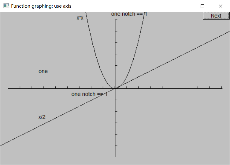
This is acceptable, although for aesthetic reasons we might want to leave some margin at the top to align with the bottom and sides, it might be a better idea to move the x-axis labels further to the left - always There are many aesthetic details that need to be refined. Part of the programmer's art is knowing when to stop and spend the time on something more meaningful (like learning a new technology or sleeping). Remember: "The best is the enemy of the good".

15.3 Function

FunctionThe class definition is as follows:

typedef double Fct(double);

struct Function : Shape {
    
    
    // the function parameters are not stored
    Function(Fct f, double r1, double r2, Point orig,
        int count = 100, double xscale = 25, double yscale = 25);    
};

Function::Function(Fct f, double r1, double r2, Point xy,
                   int count, double xscale, double yscale)
// graph f(x) for x in [r1:r2) using count line segments with (0,0) displayed at xy
// x coordinates are scaled by xscale and y coordinates scaled by yscale
{
    
    
    if (r2-r1<=0) error("bad graphing range");
    if (count <=0) error("non-positive graphing count");
    double dist = (r2-r1)/count;
    double r = r1;
    for (int i = 0; i<count; ++i) {
    
    
        add(Point(xy.x+int(r*xscale),xy.y-int(f(r)*yscale)));
        r += dist;
    }
}

Functionis one Shapewhose constructor [r1, r2)evaluates countthe subfunction at equal intervals in the interval fand stores these points in Shapethe section. The ( Shapeinherited from) draw_lines()function connects the points in turn, thus approximately drawing fthe graph of the function. xscaleand yscaleare used to scale the x and y coordinates, respectively.

Note: Here, an alias is defined typedeffor "function with one doubleparameter and return " as the type of the first parameter of the constructor, so in the above example, the function and can be passed directly as parameters.doubleFctoneslopesquare

15.3.1 Default parameters

Note that Functionconstructor parameters xscaleand yscaleinitial values are given in the declaration, which are called default arguments. If no parameter value is provided by the caller, this default value will be used. For example:

Function s(one, r_min, r_max,orig, n_points, x_scale, y_scale);
Function s2(slope, r_min, r_max, orig, n_points, x_scale);  // no yscale
Function s3(square, r_min, r_max, orig, n_points);  // no xscale, no yscale
Function s4(sqrt, r_min, r_max, orig);  // no count, no xscale, no yscale

Equivalent to

Function s(one, r_min, r_max, orig, n_points, x_scale, y_scale);
Function s2(slope, r_min, r_max,orig, n_points, x_scale, 25);
Function s3(square, r_min, r_max, orig, n_points, 25, 25);
Function s4(sqrt, r_min, r_max, orig, 100, 25, 25);

Another alternative is to provide several overloaded functions:

struct Function : Shape {
    
      // alternative, not using default arguments
    Function(Fct f, double r1, double r2, Point orig, int count, double xscale, double yscale);
    // default scale of y:
    Function(Fct f, double r1, double r2, Point orig, int count, double xscale)
            :Function(f, r1, r2, orig, count, xscale, 25) {
    
    }
    // default scale of x and y:
    Function(Fct f, double r1, double r2, Point orig, int count)
            :Function(f, r1, r2, orig, count, 25) {
    
    }
    // default count and default scale of x or y:
    Function(Fct f, double r1, double r2, Point orig)
            :Function(f, r1, r2, orig, 100) {
    
    }
};

Default parameters are often used in constructors, but are applicable to all types of functions.

Note that default parameters can only be defined for parameters at the end . If a parameter has a default value, all subsequent parameters must have default values.

Remember, you don't have to provide default parameters. If you find it difficult to give a default value, leave it to the user to specify.

15.3.2 More examples

The code below adds $\sin x$ 、 $\cos x$ 、 $\ln x$ 、 $y = e^x$ 和 $\cos x + \frac{x}{2}$ Images of several functions:

Draw a simple function graph

more examples

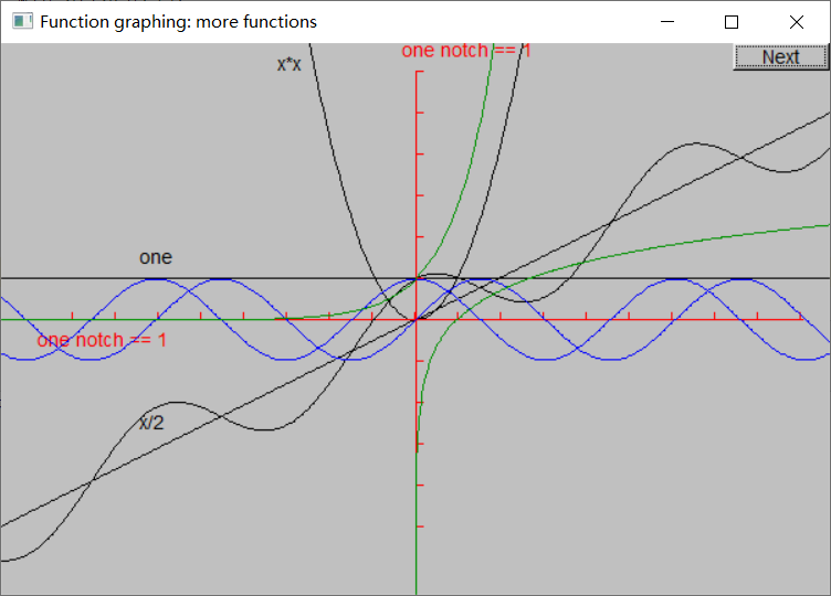
sin(), cos(), sqrt()and other standard mathematical functions are declared in the header file <cmath>.

15.3.3 Lambda expressions

Defining a function that is only passed as an argument is redundant. Therefore, C++11 introduces Lambda expressions , which are used to act as a function where the parameters are required. For example, it can be defined like this sloping_cos:

Function s5([](double x) {
    
     return cos(x) + slope(x); }, r_min, r_max, orig, n_points, x_scale, y_scale);

Among them, [](double x) { return cos(x) + slope(x); }is a Lambda expression, that is, an unnamed function. Lambda expressions consist of three parts: []a capture list (used to refer to variables in the current scope), ()a parameter list, {}and a function body. The return type can be deduced from the function body or specified explicitly: [](double x) -> double { return cos(x) + slope(x); }.

If the body of the function cannot fit within a line or two, we recommend using named functions.

See Section 21.4.3 for details on capture lists.

Note: A lambda expression without capture can be converted to a function pointer, but a lambda expression with capture cannot. So the lambda expressions above can be passed to parameters of type double(double)(ie Fct) or , but not.double (*)(double)[n](double x) { return x + n; }

15.4 Axis

When we display data, we need to use axes. One Axisconsists of a line, a series of ticks on the line, and a text label.

struct Axis : Shape {
    
    
    enum Orientation {
    
     x, y, z };
    Axis(Orientation d, Point xy, int length,
        int number_of_notches=0, string label = "");

    void draw_lines() const override;
    void move(int dx, int dy) override;
    void set_color(Color c);

    Text label;
    Lines notches;
};

The labelsum notchesobject is public so that the user can manipulate it directly, such as setting a different color for the tick than the line or moving the label. Axisis an example of an object that consists of several semi-independent objects.

AxisThe constructor of is responsible for placing a line and adding ticks:

Axis::Axis(Orientation d, Point xy, int length, int n, string lab) :
    label(Point(0,0),lab)
{
    
    
    if (length<0) error("bad axis length");
    switch (d){
    
    
    case Axis::x:
    {
    
    
        Shape::add(xy); // axis line
        Shape::add(Point(xy.x+length,xy.y));

        if (0<n) {
    
          // add notches
            int dist = length/n;
            int x = xy.x+dist;
            for (int i = 0; i<n; ++i) {
    
    
                notches.add(Point(x,xy.y),Point(x,xy.y-5));
                x += dist;
            }
        }
        // label under the line
        label.move(length/3,xy.y+20);
        break;
    }
    case Axis::y:
    {
    
    
        Shape::add(xy); // a y-axis goes up
        Shape::add(Point(xy.x,xy.y-length));

        if (0<n) {
    
          // add notches
            int dist = length/n;
            int y = xy.y-dist;
            for (int i = 0; i<n; ++i) {
    
    
                notches.add(Point(xy.x,y),Point(xy.x+5,y));
                y -= dist;
            }
        }
        // label at top
        label.move(xy.x-10,xy.y-length-10);
        break;
    }
    case Axis::z:
        error("z axis not implemented");
    }
}

Note that we Shape::add()store the two endpoints of the line in the (using) Axissection Shape, while we store the ticks in a separate Linesobject ( notches). In this way, we can manipulate the line and ticks independently, for example setting different colors.

Since Axisthere are three parts, functions must be provided when we want to manipulate it as a whole.

void Axis::draw_lines() const
{
    
    
    Shape::draw_lines();
    notches.draw();  // the notches may have a different color from the line
    label.draw();    // the label may have a different color from the line
}

void Axis::set_color(Color c)
{
    
    
    Shape::set_color(c);
    notches.set_color(c);
    label.set_color(c);
}

void Axis::move(int dx, int dy)
{
    
    
    Shape::move(dx,dy);
    notches.move(dx,dy);
    label.move(dx,dy);
}

We use draw()instead draw_lines()to draw notchesand labelto be able to use their respective colors. While the color of the line is stored in Shape, is Shape::draw()used.

Note: Since Shape::set_color()it is not a virtual function, Axis::set_color()it hides (rather than covers) the functions of the base class and cannot be Shapecalled through pointers or references Axis::set_color().

15.5 approximation

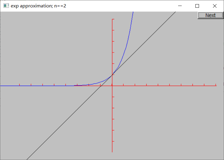
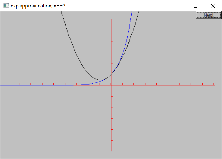
This section gives another example of a drawing function: the computation of a "dynamic" exponential function.

One way to compute exponential functions is to compute Taylor series:

$e^x = \sum_{n=0}^{\infty} \frac{x^n}{n!} = 1 + x + \frac{x^2}{2!} + \frac{x^3}{3!} + ...$

The more terms we calculate, the more precise the value of ex we ^get . What we're going to do is compute this sequence and graphically display the result after computing each term. That is, we want to plot the following functions in order:

exp0(x) = 0      // no terms
exp1(x) = 1      // one term
exp2(x) = 1 + x  // two terms
exp3(x) = 1 + x + x^2/2!
exp4(x) = 1 + x + x^2/2! + x^3/3!
exp5(x) = 1 + x + x^2/2! + x^3/3! + x^4/4!
...

Each function is a better approximation of ^ex than the previous one .

exponential function approximation

There is no factorial function in the standard library, so we have to define it ourselves. With that , the nth term of the calculation series fac()can be used . term()With that term(), you can use expe()the sum of the first n items to be calculated, which is the nth approximation function above.

From a programming standpoint, expe()the difficulty to use is Functionthat functions that only accept one parameter expe()have two. In C++, there is currently no perfect solution to this problem. A simple, imperfect solution is used here: use a global variable expN_number_of_termsto represent the precision n, and define another function expN()as Functiona parameter:

int expN_number_of_terms = 10;

double expN(double x) {
    
    
    return expe(x, expN_number_of_terms);
}

Note:

Some parameters of functions can be used std::functionand fixed in C++11 , but this cannot be converted to the required function pointer type.std::bindFunction
The code in the second edition book uses Lambda expressions [n](double x) { return expe(x, n); }. But this is wrong because lambda expressions with captures cannot be converted to function pointers: "no known conversion for argument 1 from 'main()::<lambda(double)>' to 'double (*)(double) '". Unless the type Fctis changed using Fct = std::function<double(double)>;, but this can not directly use exp()the standard library functions as parameters, because these functions have floatand doubletwo overloaded versions: "no known conversion for argument 1 from '<unresolved overloaded function type>' to 'Graph_lib: :Fct' {aka 'std::function<double(double)>'}".

The graph can now be generated. The axes and the true exponential function are provided first, and then a series of approximate functions are plotted through a loop. Note the loop at the end detach(e). FunctionThe scope of the object eis forin the loop body, and it will be destroyed after each loop, so detach(e)it is guaranteed that the window will not draw a destroyed object.

Here are the approximate results for n = 0, 1, …, 10:

Exponential function approximation (n=0)

Exponential function approximation (n=1)

Exponential function approximation (n=2)

Exponential function approximation (n=3)

Exponential function approximation (n=10)

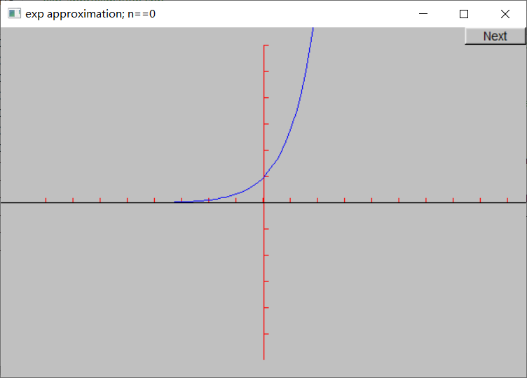
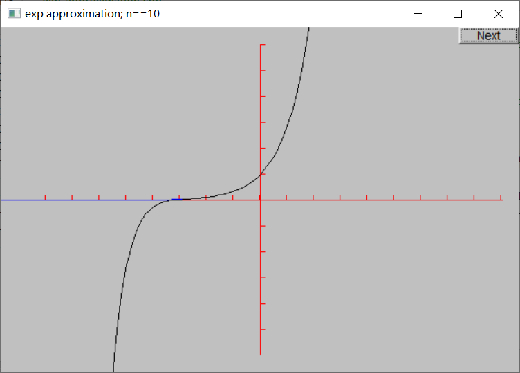
It seems that the more terms computed, the better the approximation. However, there is a limit to this, and strange things start to happen after more than 13 items. First, the approximation starts to get worse, and some vertical lines appear at item 18:

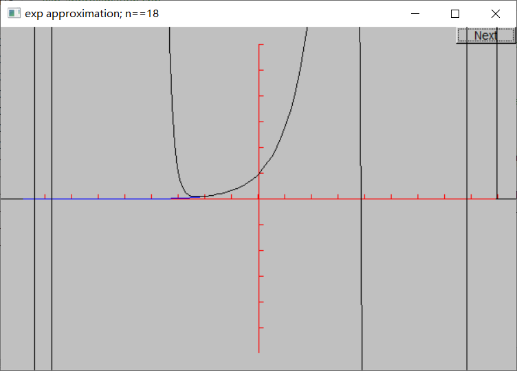
Exponential function approximation (n=18)

Remember, computer arithmetic isn't pure mathematics -- doubleit's just an approximation of real numbers, and intputting too large integers in will overflow. The reason for this phenomenon is fac()that the result exceeds intthe maximum range of (12! < 2 ³¹ -1 < 13!). This problem can be solved by changing fac()the return value type of :double

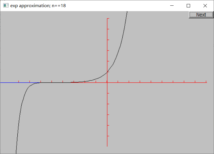
Exponential function approximation (n=18) correction

The last image (before correction) is a good illustration of the principle that "looking right" is not the same as "passing the test" . Before giving a program to others for use, test it beyond what initially seemed reasonable. Unless you have a deep understanding of the program, running it slightly longer or using slightly different data can cause the program to mess up-as in this example.

15.6 Plotting data

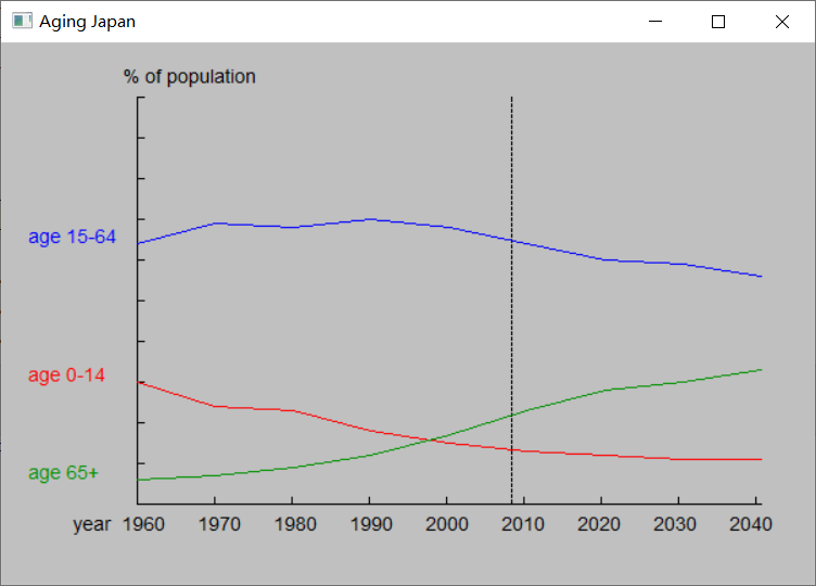
The examples in this section show data read from a file, as shown in the figure below. These data represent the age composition of the Japanese population for nearly a century, and the data to the right of the dotted line (2008) are projected.

Mapping Japanese age composition

We'll use this example to discuss the programming issues involved in displaying this kind of data:

read file
Scale data to fit window size
Display Data
label the graph

15.6.1 Reading files

The age distribution file consists of lines like this:

( 1960 : 30 64 6 )
(1970 : 24 69 7 )
(1980 : 23 68 9 )

The first number after the colon is the percentage of children (0-14 years old) in the total population, the second is the percentage of adults (15-64 years old), and the third is the percentage of the elderly (over 65 years old) .

To simplify the task of reading data, we define a type that holds data items Distributionand an input operator that reads these data items.

struct Distribution {
    
    
    int year, young, middle, old;
};

// assume format: ( year : young middle old )
istream& operator>>(istream& is, Distribution& d) {
    
    
    char ch1 = 0, ch2 = 0, ch3 = 0;
    Distribution dd;

    if (!(is >> ch1 >> dd.year >> ch2 >> dd.young >> dd.middle >> dd.old >> ch3))
        return is;
    else if (ch1 != '(' || ch2 != ':' || ch3 != ')') {
    
    
        is.clear(ios_base::failbit);
        return is;
    }

    d = dd;
    return is;
}

This is a direct application of the ideas in Section 10.9. We use Distributiontypes and >>operators to divide the code into logical parts, which facilitates understanding and debugging. We define types to make the code more directly correspond to the way we think about concepts.

15.6.2 General layout

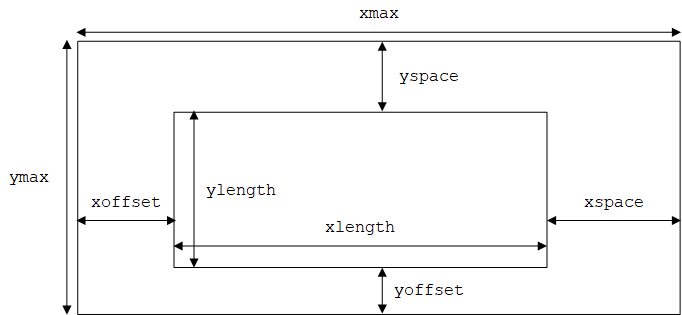
Getting drawing code to be both correct and beautiful is tricky. The main reason is that we have to do a lot of high precision calculations about sizes and offsets. To simplify, we first define a set of symbolic constants to represent how we use screen space:

constexpr int xmax = 600;       // window size
constexpr int ymax = 400;

constexpr int xoffset = 100;    // distance from left-hand side of window to y axis
constexpr int yoffset = 60;     // distance from bottom of window to x axis

constexpr int xspace = 40;      // space beyond axis
constexpr int yspace = 40;

constexpr int xlength = xmax - xoffset - xspace;    // length of axes
constexpr int ylength = ymax - yoffset - yspace;

This defines a rectangular space (window) and another rectangle inside (defined by the coordinate axes), as shown in the figure below.

screen layout

15.6.3 Scaling data

Next you need to define how to fit the data into this space. We scale the data to fit the space defined by the axes, for which we need the scaling factor, which is the ratio between the extent of the data and the extent of the axes:

constexpr double xscale = double(xlength) / (end_year - base_year);
constexpr double yscale = double(ylength) / 100;

Note that the scaling factors ( xscaleand yscale) must be floating point numbers, otherwise the calculation will suffer from severe rounding errors.

Year and age scales can be converted to x-coordinates and y-coordinates respectively in the same way:

x = xoffset + (year - base_year) * xscale
y = yoffset + (percent - 0) * yscale

To simplify the code and minimize the chance of errors, we define a small class to perform this calculation:

// data value to coordinate conversion
class Scale {
    
    
    int cbase;  // coordinate base
    int vbase;  // base of values
    double scale;

public:
    Scale(int b, int vb, double s) :cbase(b), vbase(vb), scale(s) {
    
    }
    int operator()(int v) const {
    
     return cbase + (v - vbase) * scale; }
};

ScaleThe class is responsible for [vbase, +∞)mapping the range to [cbase, +∞)and scaling scale. That is, to give v, to seek c, to make c - cbase = (v - vbase) * scale.

So you can define:

Scale xs(xoffset, base_year, xscale);
Scale ys(ymax - yoffset, 0, -yscale);

Note that we make ysthe scaling factor negative to reflect that the window's y-coordinate grows downward.

Years can now xsbe converted to x-coordinates and yspercentages to y-coordinates using:

int x = xs(d.year);
int y = ys(d.young);

Since Scaleclasses overload ()operators, xsand yscan be called like functions.

15.6.4 Constructing images

Finally, we can write the drawing code. First create the window and place the axes:

Graph_lib::Window win(Point(100, 100), xmax, ymax, "Aging Japan");

Axis x_axis(
        Axis::x, Point(xoffset, ymax - yoffset), xlength, (end_year - base_year) / 10,
        "year  1960      1970      1980      1990      "
        "2000      2010      2020      2030      2040");
x_axis.label.move(-100, 0);

Axis y_axis(Axis::y, Point(xoffset, ymax - yoffset), ylength, 10, "% of population");

Line current_year(Point(xs(2008), ys(0)), Point(xs(2008), ys(100)));
current_year.set_style(Line_style::dash);

The intersection point of the coordinate axes Point(xoffset, ymax - yoffset)represents (1960, 0). Each tick on the y-axis represents 10% of the population, and each tick on the x-axis represents 10 years.

Note the string format of the x-axis labels: two adjacent string constants are concatenated by the compiler , which is a useful trick for laying out long string constants to make code more readable.

current_yearis a vertical line separating known and predicted data.

With the axes in place, we can work with the data. Can be used Open_polylineto draw a line chart. Define three Open_polyline, and fill them with data in a read loop:

Open_polyline children;
Open_polyline adults;
Open_polyline aged;

for (Distribution d; ifs >> d;) {
    
    
    if (d.year < base_year || d.year > end_year)
        error("year out of range");
    if (d.young + d.middle + d.old != 100)
        error("percentages don't add up");
    const int x = xs(d.year);
    children.add(Point(x, ys(d.young)));
    adults.add(Point(x, ys(d.middle)));
    aged.add(Point(x, ys(d.old)));
}

To make the graphs more readable, we label and color each graph:

Text children_label(Point(20, children.point(0).y), "age 0-14");
children.set_color(Color::red);
children_label.set_color(Color::red);

Text adults_label(Point(20, adults.point(0).y), "age 15-64");
adults.set_color(Color::blue);
adults_label.set_color(Color::blue);

Text aged_label(Point(20, aged.point(0).y), "age 65+");
aged.set_color(Color::dark_green);
aged_label.set_color(Color::dark_green);

Finally attach all Shapeobjects to Windowand start the GUI system:

win.attach(x_axis);
win.attach(y_axis);
win.attach(current_year);

win.attach(children);
win.attach(adults);
win.attach(aged);

win.attach(children_label);
win.attach(adults_label);
win.attach(aged_label);

gui_main();

The gui_main()function is declared in Window.h, and its function is to enter the FLTK main loop, similar to Simple_window::wait_for_button().

Complete code: Drawing Japanese age composition

The final effect is shown in the figure below: