1. Prepare the dataset
One hundred and two types of flower data set download

flower_data includes train and valid files, which store 102 files respectively, corresponding to 102 types of flowers
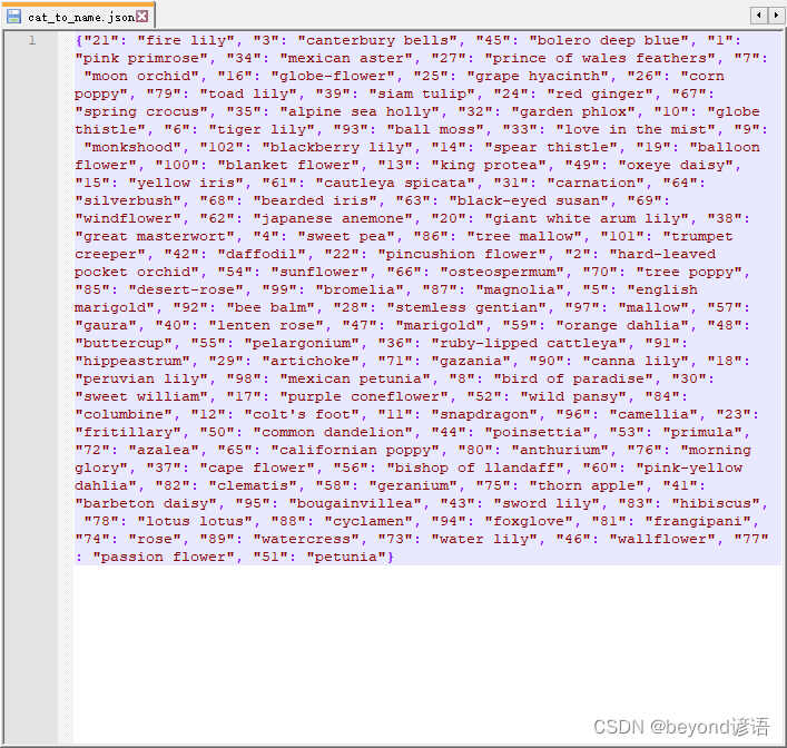
cat_to_name.json is the category and flower variety key-value pair,
decompress the compressed package, and put it in the same place as the project class path

Second, guide package
If you encounter an error report and there is no xxx package, pip install xxxjust enter the relevant environment directly.
import os
import imageio
import time
import warnings
import random
import sys
import copy
import json
import numpy as np
import matplotlib.pyplot as plt
import torch
from torch import nn
import torch.optim as optim
import torchvision
from PIL import Image
from torchvision import transforms, models, datasets
%matplotlib inline
%matplotlib inlineThe drawing can be embedded in the notebook, and can be omittedplt.show()
3. Read the dataset
train_dir : training set path
valid_dir : validation set path
data_dir = './flower_data/'
train_dir = data_dir + '/train'
valid_dir = data_dir + '/valid'
Four, transforms module - data preprocessing
Data Augmentation Data Augmentation
performs random rotation, center cropping, horizontal flipping, vertical flipping, changing brightness, contrast, saturation, hue, changing grayscale, standardization and other operations on the data set in order to expand the data set
Different preprocessing methods are used for the data under the train and valid folders
data_transforms = {


    'train': transforms.Compose([transforms.RandomRotation(45),#随机旋转,-45到45度之间随机选
        transforms.CenterCrop(224),#从中心开始裁剪
        transforms.RandomHorizontalFlip(p=0.5),#随机水平翻转 选择一个概率概率
        transforms.RandomVerticalFlip(p=0.5),#随机垂直翻转
        transforms.ColorJitter(brightness=0.2, contrast=0.1, saturation=0.1, hue=0.1),#参数1为亮度,参数2为对比度,参数3为饱和度,参数4为色相
        transforms.RandomGrayscale(p=0.025),#概率转换成灰度率,3通道就是R=G=B
        transforms.ToTensor(),
        transforms.Normalize([0.485, 0.456, 0.406], [0.229, 0.224, 0.225])#均值,标准差
    ]),
    'valid': transforms.Compose([transforms.Resize(256),
        transforms.CenterCrop(224),#从中心开始裁剪
        transforms.ToTensor(),
        transforms.Normalize([0.485, 0.456, 0.406], [0.229, 0.224, 0.225])
    ]),
}
5. ImageFolder module - make Batch data set
Official website API: torchvision.datasets.ImageFolder
image_datasets = {x: datasets.ImageFolder(os.path.join(data_dir, x), data_transforms[x]) for x in ['train', 'valid']} reads the data set structure
xas a folder, including train and valid
data_transforms[x]Data set preprocessing Data enhancement performs different preprocessing on train and valid
batch_size = 8

image_datasets = {

    x: datasets.ImageFolder(os.path.join(data_dir, x), data_transforms[x]) for x in ['train', 'valid']}
dataloaders = {

    x: torch.utils.data.DataLoader(image_datasets[x], batch_size=batch_size, shuffle=True) for x in ['train', 'valid']}
dataset_sizes = {

    x: len(image_datasets[x]) for x in ['train', 'valid']}
class_names = image_datasets['train'].classes


image_datasets
"""
{'train': Dataset ImageFolder
     Number of datapoints: 6552
     Root location: ./flower_data/train
     StandardTransform
 Transform: Compose(
                RandomRotation(degrees=[-45.0, 45.0], interpolation=nearest, expand=False, fill=0)
                CenterCrop(size=(224, 224))
                RandomHorizontalFlip(p=0.5)
                RandomVerticalFlip(p=0.5)
                ColorJitter(brightness=(0.8, 1.2), contrast=(0.9, 1.1), saturation=(0.9, 1.1), hue=(-0.1, 0.1))
                RandomGrayscale(p=0.025)
                ToTensor()
                Normalize(mean=[0.485, 0.456, 0.406], std=[0.229, 0.224, 0.225])
            ),
 'valid': Dataset ImageFolder
     Number of datapoints: 818
     Root location: ./flower_data/valid
     StandardTransform
 Transform: Compose(
                Resize(size=256, interpolation=bilinear, max_size=None, antialias=warn)
                CenterCrop(size=(224, 224))
                ToTensor()
                Normalize(mean=[0.485, 0.456, 0.406], std=[0.229, 0.224, 0.225])
            )}
"""


dataloaders
"""
{'train': <torch.utils.data.dataloader.DataLoader at 0x1924ed088e0>,
 'valid': <torch.utils.data.dataloader.DataLoader at 0x19264e750d0>}
"""


dataset_sizes
"""
{'train': 6552, 'valid': 818}
"""
6. Read the cat_to_name.json file
The cat_to_name.json file indicates that the label model corresponding to each type of flower
is predicted. In fact, the probability value of each category is first obtained, and then the largest value is selected to find the corresponding category. At this time, only the category number is obtained. Through the json file, the flower name of the actual category corresponding to the number can be extracted
with open('cat_to_name.json', 'r') as f:
    cat_to_name = json.load(f)

cat_to_name
"""
{'21': 'fire lily',
 '3': 'canterbury bells',
 '45': 'bolero deep blue',
 '1': 'pink primrose',
 '34': 'mexican aster',
 '27': 'prince of wales feathers',
 '7': 'moon orchid',
 ......
 '77': 'passion flower',
 '51': 'petunia'}
"""
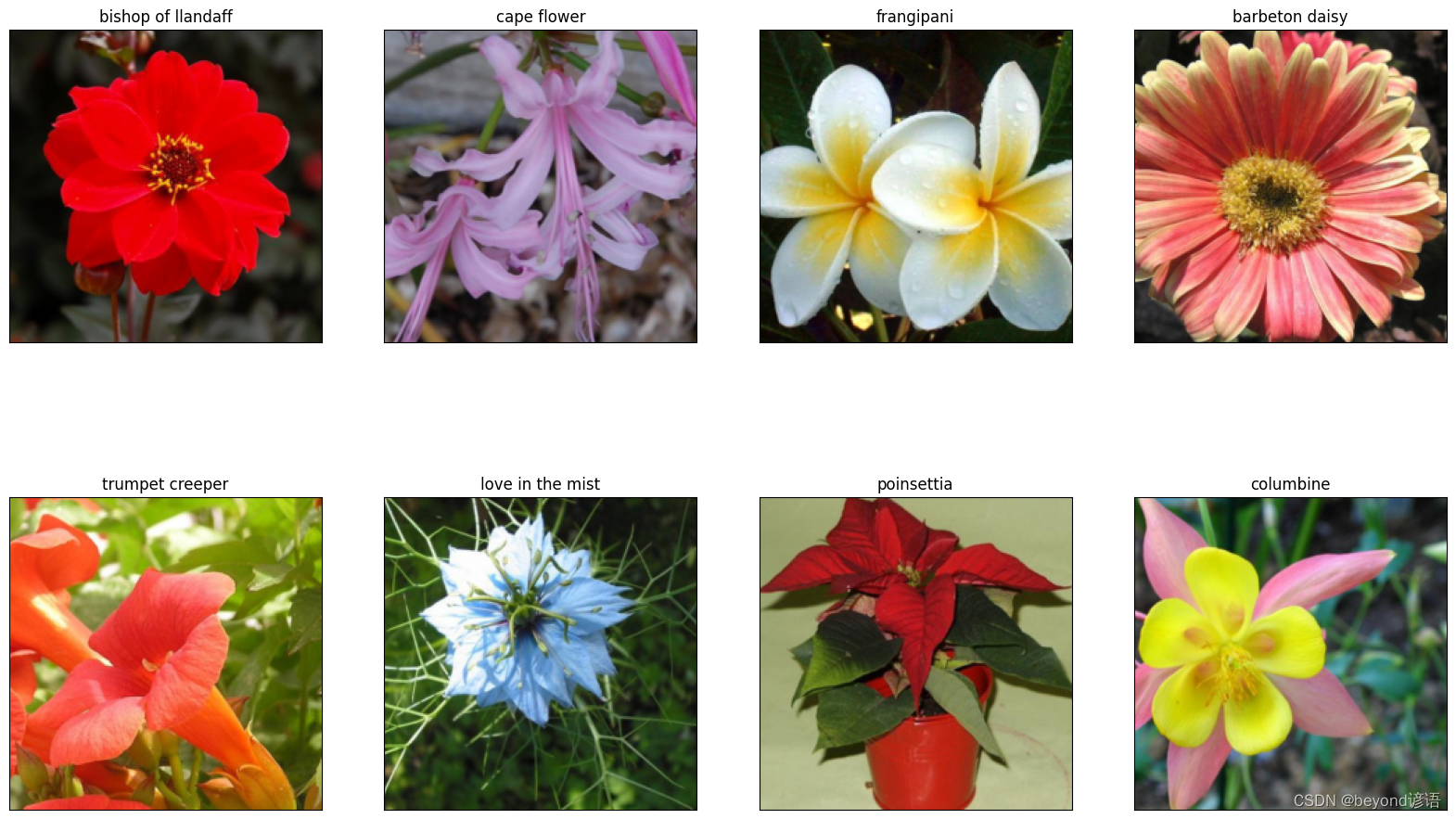
Seven, display data set
The data in torch is [C, H, W], while the data in PIL is [H, W, C]. Therefore, by image.transpose(1,2,0)converting the format,
the data preprocessing is to subtract the mean value and divide it by the standard deviation , (x-均值)/标准差 = y
and to restore it needs to be multiplied The standard deviation plus the mean , (y * 标准差) + 均值 = xieimage * np.array((0.229, 0.224, 0.225)) + np.array((0.485, 0.456, 0.406))
def im_convert(tensor):
    """ 展示数据"""

    image = tensor.to("cpu").clone().detach()
    image = image.numpy().squeeze()
    image = image.transpose(1,2,0)
    image = image * np.array((0.229, 0.224, 0.225)) + np.array((0.485, 0.456, 0.406))
    image = image.clip(0, 1)

    return image
fig=plt.figure(figsize=(20, 12))
columns = 4
rows = 2

dataiter = iter(dataloaders['valid'])
inputs, classes = next(dataiter)

for idx in range (columns*rows):
    ax = fig.add_subplot(rows, columns, idx+1, xticks=[], yticks=[])
    ax.set_title(cat_to_name[str(int(class_names[classes[idx]]))])
    plt.imshow(im_convert(inputs[idx]))
plt.show()
Eight, transfer learning
Small data sets will lead to over-fitting of the model; transfer learning can use model parameters that have been trained by others. Fully connected layer FC, the layer used by oneself; the weight parameter is not updated, which means that the ability to extract features will not change. If other people's network is good, just use other people's weight parameters.
Official website API: Models and pre-trained weights
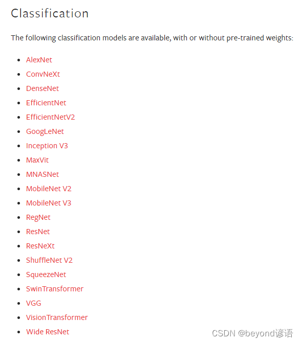
Here, the resnet152 network model is used as an example. When transferring learning, not all weight parameters of others are used.
This task is 1000 classifications [2048,1000], so (fc): Linear(in_features=2048, out_features=1000, bias=True)
this project is a classification task of 102 categories, so it is necessary to modify all Change to the connection layer Although [2048,102]
the resnet152 network model has been obtained, the task requirements are different, and you need to modify it according to the actual situation of your task. There is only one fully connected layer here, so you only need to modify this fully connected layer.
model_name = 'resnet'  #可选的比较多 ['resnet', 'alexnet', 'vgg', 'squeezenet', 'densenet', 'inception']
#是否用人家训练好的特征来做
feature_extract = True


# 是否用GPU训练
train_on_gpu = torch.cuda.is_available()

if not train_on_gpu:
    print('CUDA is not available.  Training on CPU ...')
else:
    print('CUDA is available!  Training on GPU ...')

device = torch.device("cuda:0" if torch.cuda.is_available() else "cpu")
Selectively freeze certain network layers, and their corresponding weight parameters will not be updated
def set_parameter_requires_grad(model, feature_extracting):
    if feature_extracting:
        for param in model.parameters():
            param.requires_grad = False
model_ft = models.resnet152()
model_ft #看一下resnet152网络模型架构
"""
ResNet(
  (conv1): Conv2d(3, 64, kernel_size=(7, 7), stride=(2, 2), padding=(3, 3), bias=False)
  (bn1): BatchNorm2d(64, eps=1e-05, momentum=0.1, affine=True, track_running_stats=True)
  (relu): ReLU(inplace=True)
  (maxpool): MaxPool2d(kernel_size=3, stride=2, padding=1, dilation=1, ceil_mode=False)
  (layer1): Sequential(
    (0): Bottleneck(
      (conv1): Conv2d(64, 64, kernel_size=(1, 1), stride=(1, 1), bias=False)
      ......
(avgpool): AdaptiveAvgPool2d(output_size=(1, 1))
  (fc): Linear(in_features=2048, out_features=1000, bias=True)
)
"""
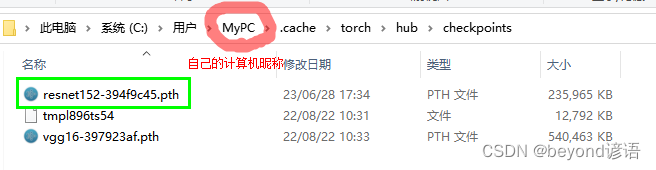
models.resnet152(pretrained=use_pretrained)Indicates whether to download the pre-training weight file, and if so, it use_pretrained=Truewill be downloaded online. The default download path is: C:\Users\MyPC\.cache\torch\hub\checkpoints, where MyPC is my computer name
num_ftrs = model_ft.fc.in_featuresto get the fully connected layer
model_ft.fc = nn.Sequential(nn.Linear(num_ftrs, 102), nn.LogSoftmax(dim=1))and modify the fully connected layer. The previous one was 1000 categories, now Change to 102 classification
def initialize_model(model_name, num_classes, feature_extract, use_pretrained=True):
    # 选择合适的模型,不同模型的初始化方法稍微有点区别
    model_ft = None
    input_size = 0

    if model_name == "resnet":
        """ Resnet152
        """
        model_ft = models.resnet152(pretrained=use_pretrained)
        set_parameter_requires_grad(model_ft, feature_extract)
        num_ftrs = model_ft.fc.in_features
        model_ft.fc = nn.Sequential(nn.Linear(num_ftrs, 102),
                                   nn.LogSoftmax(dim=1))
        input_size = 224

    elif model_name == "alexnet":
        """ Alexnet
        """
        model_ft = models.alexnet(pretrained=use_pretrained)
        set_parameter_requires_grad(model_ft, feature_extract)
        num_ftrs = model_ft.classifier[6].in_features
        model_ft.classifier[6] = nn.Linear(num_ftrs,num_classes)
        input_size = 224

    elif model_name == "vgg":
        """ VGG11_bn
        """
        model_ft = models.vgg16(pretrained=use_pretrained)
        set_parameter_requires_grad(model_ft, feature_extract)
        num_ftrs = model_ft.classifier[6].in_features
        model_ft.classifier[6] = nn.Linear(num_ftrs,num_classes)
        input_size = 224

    elif model_name == "squeezenet":
        """ Squeezenet
        """
        model_ft = models.squeezenet1_0(pretrained=use_pretrained)
        set_parameter_requires_grad(model_ft, feature_extract)
        model_ft.classifier[1] = nn.Conv2d(512, num_classes, kernel_size=(1,1), stride=(1,1))
        model_ft.num_classes = num_classes
        input_size = 224

    elif model_name == "densenet":
        """ Densenet
        """
        model_ft = models.densenet121(pretrained=use_pretrained)
        set_parameter_requires_grad(model_ft, feature_extract)
        num_ftrs = model_ft.classifier.in_features
        model_ft.classifier = nn.Linear(num_ftrs, num_classes)
        input_size = 224

    elif model_name == "inception":
        """ Inception v3
        Be careful, expects (299,299) sized images and has auxiliary output
        """
        model_ft = models.inception_v3(pretrained=use_pretrained)
        set_parameter_requires_grad(model_ft, feature_extract)
        # Handle the auxilary net
        num_ftrs = model_ft.AuxLogits.fc.in_features
        model_ft.AuxLogits.fc = nn.Linear(num_ftrs, num_classes)
        # Handle the primary net
        num_ftrs = model_ft.fc.in_features
        model_ft.fc = nn.Linear(num_ftrs,num_classes)
        input_size = 299

    else:
        print("Invalid model name, exiting...")
        exit()

    return model_ft, input_size
Summary: Migration learning steps
①Get the network model, and specify use_pretrained= True whether to use the weight parameters of the model trained by others
②You can choose whether to freeze some layers according to the actual situation, that is, you don’t need to ask for the gradient when the gradient is updated , that is, param.requires_grad = False
③ modify the last fully connected layer of the network to be consistent with its own task
先训练自己的,保持别人的网络权重参数不变 然后在之前训练的基础上,继续训练整体的网络模型,对整体网络模型权重参数进行微调,这样的效果最好
Nine, network model parameter settings
Specify which layers need to be trained
model_name = 'resnet'and select the resnet152 network model.
The final output result is 102 categories
feature_extract. Do you want to freeze some layers
use_pretrainedor use the model weight parameters that have been trained by others?
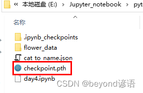
filename='checkpoint.pth'Name the trained weight parameter as checkpoint.pth and save it to the current path
model_ft, input_size = initialize_model(model_name, 102, feature_extract, use_pretrained=True)

#GPU计算
model_ft = model_ft.to(device)

# 模型保存
filename='checkpoint.pth'

# 是否训练所有层
params_to_update = model_ft.parameters()
print("Params to learn:")
if feature_extract:
    params_to_update = []
    for name,param in model_ft.named_parameters():
        if param.requires_grad == True:
            params_to_update.append(param)
            print("\t",name)
else:
    for name,param in model_ft.named_parameters():
        if param.requires_grad == True:
            print("\t",name)
"""
Params to learn:
	 fc.0.weight
	 fc.0.bias
"""
It can be seen that Linear(in_features=2048, out_features=102, bias=True)the fully connected layer has been modified, and it is classified according to the actual situation of its own task 102
model_ft
"""
ResNet(
  (conv1): Conv2d(3, 64, kernel_size=(7, 7), stride=(2, 2), padding=(3, 3), bias=False)
  (bn1): BatchNorm2d(64, eps=1e-05, momentum=0.1, affine=True, track_running_stats=True)
  (relu): ReLU(inplace=True)
  (maxpool): MaxPool2d(kernel_size=3, stride=2, padding=1, dilation=1, ceil_mode=False)
  (layer1): Sequential(
    (0): Bottleneck(
      (conv1): Conv2d(64, 64, kernel_size=(1, 1), stride=(1, 1), bias=False)
      ......
  (avgpool): AdaptiveAvgPool2d(output_size=(1, 1))
  (fc): Sequential(
    (0): Linear(in_features=2048, out_features=102, bias=True)
    (1): LogSoftmax(dim=1)
  )
)
"""
10. Optimizer parameter settings
Generally, the Adam optimizer works well, and
optim.Adam(params_to_update, lr=1e-2)the learning rate set initially is not too small. If lr=0.01,
the learning rate decay strategy is used later to make the learning rate gradually decrease.optim.lr_scheduler.StepLR(optimizer_ft, step_size=7, gamma=0.1)
# 优化器设置
optimizer_ft = optim.Adam(params_to_update, lr=1e-2)
scheduler = optim.lr_scheduler.StepLR(optimizer_ft, step_size=7, gamma=0.1)#学习率每7个epoch衰减成原来的1/10
#最后一层已经LogSoftmax()了,所以不能nn.CrossEntropyLoss()来计算了,nn.CrossEntropyLoss()相当于logSoftmax()和nn.NLLLoss()整合
criterion = nn.NLLLoss()
11. Training module parameter setting
is_inceptionWhether to use additional other networks, it is enough to use resnet152 here.
Each epoch saves the model with the highest accuracy rate, which is convenient for subsequent training.
def train_model(model, dataloaders, criterion, optimizer, num_epochs=25, is_inception=False,filename=filename):
    since = time.time()
    best_acc = 0 #保存一个最好的准确率
    """
    checkpoint = torch.load(filename)
    best_acc = checkpoint['best_acc']
    model.load_state_dict(checkpoint['state_dict'])
    optimizer.load_state_dict(checkpoint['optimizer'])
    model.class_to_idx = checkpoint['mapping']
    """
    model.to(device)

    val_acc_history = []
    train_acc_history = []
    train_losses = []
    valid_losses = []
    LRs = [optimizer.param_groups[0]['lr']]

    best_model_wts = copy.deepcopy(model.state_dict())

    for epoch in range(num_epochs):
        print('Epoch {}/{}'.format(epoch, num_epochs - 1))
        print('-' * 10)

        # 训练和验证
        for phase in ['train', 'valid']:
            if phase == 'train':
                model.train()  # 训练
            else:
                model.eval()   # 验证

            running_loss = 0.0
            running_corrects = 0

            # 把数据都取个遍
            for inputs, labels in dataloaders[phase]:
                inputs = inputs.to(device)
                labels = labels.to(device)

                # 清零
                optimizer.zero_grad()
                # 只有训练的时候计算和更新梯度
                with torch.set_grad_enabled(phase == 'train'):
                    if is_inception and phase == 'train':
                        outputs, aux_outputs = model(inputs)
                        loss1 = criterion(outputs, labels)
                        loss2 = criterion(aux_outputs, labels)
                        loss = loss1 + 0.4*loss2
                    else:#resnet执行的是这里
                        outputs = model(inputs)
                        loss = criterion(outputs, labels)

                    _, preds = torch.max(outputs, 1)

                    # 训练阶段更新权重
                    if phase == 'train':
                        loss.backward()
                        optimizer.step()

                # 计算损失
                running_loss += loss.item() * inputs.size(0)
                running_corrects += torch.sum(preds == labels.data)

            epoch_loss = running_loss / len(dataloaders[phase].dataset)
            epoch_acc = running_corrects.double() / len(dataloaders[phase].dataset)


            time_elapsed = time.time() - since
            print('Time elapsed {:.0f}m {:.0f}s'.format(time_elapsed // 60, time_elapsed % 60))
            print('{} Loss: {:.4f} Acc: {:.4f}'.format(phase, epoch_loss, epoch_acc))


            # 得到最好那次的模型
            if phase == 'valid' and epoch_acc > best_acc:
                best_acc = epoch_acc
                best_model_wts = copy.deepcopy(model.state_dict())
                state = {


                  'state_dict': model.state_dict(),
                  'best_acc': best_acc,
                  'optimizer' : optimizer.state_dict(),
                }
                torch.save(state, filename)
            if phase == 'valid':
                val_acc_history.append(epoch_acc)
                valid_losses.append(epoch_loss)
                scheduler.step(epoch_loss)
            if phase == 'train':
                train_acc_history.append(epoch_acc)
                train_losses.append(epoch_loss)

        print('Optimizer learning rate : {:.7f}'.format(optimizer.param_groups[0]['lr']))
        LRs.append(optimizer.param_groups[0]['lr'])
        print()

    time_elapsed = time.time() - since
    print('Training complete in {:.0f}m {:.0f}s'.format(time_elapsed // 60, time_elapsed % 60))
    print('Best val Acc: {:4f}'.format(best_acc))

    # 训练完后用最好的一次当做模型最终的结果
    model.load_state_dict(best_model_wts)
    return model, val_acc_history, train_acc_history, valid_losses, train_losses, LRs
12. Model training
① First freeze other people's network weight parameters, and only train the parameters of the fully connected layer
The training here is equivalent to only training the last fully connected layer, and other people's network weight parameters have been frozen, relatively speaking, the training speed is faster
If the computer configuration is low, num_epochs=20the training times can be changed to a smaller number
model_ft, val_acc_history, train_acc_history, valid_losses, train_losses, LRs = train_model(model_ft, dataloaders, criterion, optimizer_ft, num_epochs=20, is_inception=(model_name=="inception"))
②Continue to train all layers on the basis of the previous network model
All the weight parameters of the network model are trained, so the learning rate is set to be smaller, just fine-tuning. At this time, all layers of training are just fine-tuning.
for param in model_ft.parameters():
    param.requires_grad = True

# 再继续训练所有的参数,学习率调小一点
optimizer = optim.Adam(params_to_update, lr=1e-4)
scheduler = optim.lr_scheduler.StepLR(optimizer_ft, step_size=7, gamma=0.1)

# 损失函数
criterion = nn.NLLLoss()
This training should continue on the previous basis, so load the model with the best accuracy before, and fine-tune the training on this basis
# Load the checkpoint

checkpoint = torch.load(filename)
best_acc = checkpoint['best_acc']
model_ft.load_state_dict(checkpoint['state_dict'])
optimizer.load_state_dict(checkpoint['optimizer'])
#model_ft.class_to_idx = checkpoint['mapping']
Model training, it will be time-consuming at this time, because it is the fine-tuning of the weight parameters of the entire model
model_ft, val_acc_history, train_acc_history, valid_losses, train_losses, LRs = train_model(model_ft, dataloaders, criterion, optimizer, num_epochs=10, is_inception=(model_name=="inception"))
After the training is completed, the weight parameters will be saved
13. Load the trained model
Load the trained model into
model_ft, input_size = initialize_model(model_name, 102, feature_extract, use_pretrained=True)

# GPU模式
#model_ft = model_ft.to(device)

# 保存文件的名字
filename='checkpoint.pth'

# 加载模型
checkpoint = torch.load(filename)
best_acc = checkpoint['best_acc']
model_ft.load_state_dict(checkpoint['state_dict'])
Fourteen, model testing
Ⅰ, test data set preprocessing
In order to test the model, the test data must be consistent with the training data set.
Normalize the test data set np.array(img)/255and compress the 0-255 pixel value to
the operation used by the test set and the training set between 0-1. The type of mean and standard deviation
is consistent in torch [C,H,W], which needs to be img.transpose((2, 0, 1))converted to[H,W,C]
def process_image(image_path):
    # 读取测试数据
    img = Image.open(image_path)
    # Resize,thumbnail方法只能进行缩小,所以进行了判断
    if img.size[0] > img.size[1]:
        img.thumbnail((10000, 256))
    else:
        img.thumbnail((256, 10000))
    # Crop操作
    left_margin = (img.width-224)/2
    bottom_margin = (img.height-224)/2
    right_margin = left_margin + 224
    top_margin = bottom_margin + 224
    img = img.crop((left_margin, bottom_margin, right_margin,
                      top_margin))
    # 相同的预处理方法
    img = np.array(img)/255
    mean = np.array([0.485, 0.456, 0.406]) #provided mean
    std = np.array([0.229, 0.224, 0.225]) #provided std
    img = (img - mean)/std

    # 注意颜色通道应该放在第一个位置
    img = img.transpose((2, 0, 1))

    return img
Ⅱ, display the test image
def imshow(image, ax=None, title=None):
    """展示数据"""
    if ax is None:
        fig, ax = plt.subplots()

    # 颜色通道还原
    image = np.array(image).transpose((1, 2, 0))

    # 预处理还原
    mean = np.array([0.485, 0.456, 0.406])
    std = np.array([0.229, 0.224, 0.225])
    image = std * image + mean
    image = np.clip(image, 0, 1)

    ax.imshow(image)
    ax.set_title(title)

    return ax
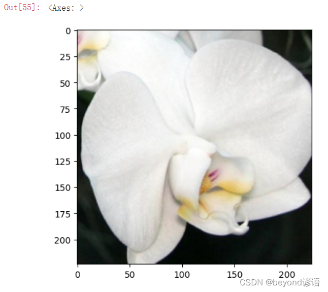
I randomly selected one from the verification set here.
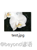
image_path = 'test.jpg'
img = process_image(image_path)
imshow(img)

img.shape # (3, 224, 224)
Ⅲ, get a batch of test data and feed it to the trained network
Here it is taken from the valid folder in the dataset
torch.Size([8, 102])Indicates that a batch in the output has 8 pieces of data, and each piece of data has 102 results, and each result corresponds to a probability value belonging to a different category
# 得到一个batch的测试数据
dataiter = iter(dataloaders['valid'])
images, labels = next(dataiter)

model_ft.eval()

if train_on_gpu:
    output = model_ft(images.cuda())
else:
    output = model_ft(images)


output.shape # torch.Size([8, 102])
Ⅳ, get the id with the highest probability value of the 8 pieces of data in a batch
_, preds_tensor = torch.max(output, 1)

preds = np.squeeze(preds_tensor.numpy()) if not train_on_gpu else np.squeeze(preds_tensor.cpu().numpy())
preds
"""
array([71, 89, 73, 54, 83, 12, 59, 78], dtype=int64)
"""
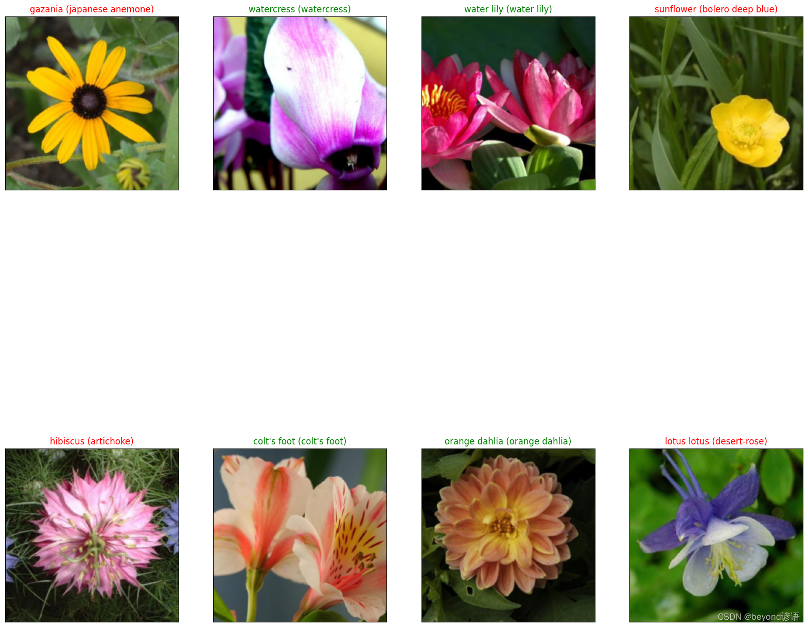
Ⅴ, display the predicted results
What you get in the previous step is only the id of the flower, which is converted to the specific name of the corresponding flower type cat_to_name[str(preds[idx])]according to the previous file . The prediction is correct, and the green label is displayed. The red label indicates that the prediction is wrong.cat_to_name.json
Label form: the model predicts the type of flower (the actual type of flower)
fig=plt.figure(figsize=(20, 20))
columns =4
rows = 2

for idx in range (columns*rows):
    ax = fig.add_subplot(rows, columns, idx+1, xticks=[], yticks=[])
    plt.imshow(im_convert(images[idx]))
    ax.set_title("{} ({})".format(cat_to_name[str(preds[idx])], cat_to_name[str(labels[idx].item())]),
                 color=("green" if cat_to_name[str(preds[idx])]==cat_to_name[str(labels[idx].item())] else "red"))
plt.show()