YOLOv3: An Incremental Improvement - Incremental Improvement (arXiv 2018)
Disclaimer: This translation is only a personal study record
Article information
- 标题:YOLOv3: An Incremental Improvement (arXiv 2018)
- 作者:Joseph Redmon, Ali Farhadi
- Article link: https://arxiv.org/pdf/1804.02767.pdf
- Article code: https://pjreddie.com/darknet/yolo/
Summary
We have some updates to YOLO! We made some small design changes to make it even better. We also trained this very large new network. It's a little bigger than last time, but more accurate. It's still fast though, don't worry. At 320×320, YOLOv3 runs in 22ms and gets 28.2mAP, which is as accurate as SSD but three times faster. When we look at the old .5 IOU mAP detection metric YOLOv3 is pretty good. On Titan X, it hits 57.9 AP50 in 51ms, compared to RetinaNet's 57.5 AP50 in 198ms , similar performance but 3.8 times faster. As always, all code is online at https://pjreddie.com/yolo/.
1 Introduction
Sometimes you're just on the phone for a year, you know? I haven't done a lot of research this year. Spent a lot of time on Twitter. Played around with GANs for a while. I have a little momentum left over from last year [12][1]; I managed to make some improvements to YOLO. But, honestly, there's nothing more interesting than that, just some small changes to make it better. I also helped others a little bit.
In fact, that's why we're here today. We have a deadline [4] for ready-to-photographs, and we need to cite some random update I made to YOLO, but we have no sources. So, get ready for a tech report!
The great thing about tech reports is that they need no introduction, you all know why we are here. Thus, the end of this Introduction will serve as a signpost for the rest of the paper. First, we will tell you what YOLOv3 does. Then we'll tell you how we do it. We'll also tell you about some of the things we've tried without success. Finally, we'll consider what this all means.
2. Processing
So the way YOLOv3 handles it is: we mostly get good ideas from other people. We also train a new classifier network that outperforms the others. We'll take you through the entire system from the ground up so you can understand everything.

Figure 1. We adjusted this figure according to the Focal Loss paper [9]. YOLOv3 runs significantly faster than other detection methods with comparable performance. Whether it's the M40 or the Titan X, they're basically the same GPU.
2.1 Bounding box prediction
Following YOLO9000, our system uses dimension clusters as anchor boxes to predict bounding boxes [15]. The network predicts 4 coordinates, t x , ty , t w , t h , for each bounding box . If the cell is offset (c x , cy ) from the top-left corner of the image , and the bounding box prior has width and height p w , ph , then the prediction corresponds to:

During training, we use squared error and loss. If the true value of a coordinate prediction is t ^ ∗ \hat{t} *t^ ∗, then our gradient is the ground truth (computed from the ground truth box) minus our prediction:t ^ ∗ − t ∗ \hat{t} *−t*t^∗− t ∗ . This truth value can be easily calculated by reversing the above equation.
YOLOv3 uses logistic regression to predict objectness scores for each bounding box. This value should be 1 if the bounding box prior overlaps the ground-truth object more than any other bounding box prior. If the bounding box prior is not the best, but does overlap the ground-truth object by more than a certain threshold, we ignore the prediction, as in [17]. We use a threshold of .5. Unlike [17], our system assigns only one bounding box prior to each ground-truth object. If the bounding box prior is not assigned to the ground-truth target, then there is no loss of coordinate or class prediction, only loss of targetness.

Figure 2. Bounding boxes with dimensionality priors and location predictions . We predict the box width and height as offsets from the cluster centroids. We use the sigmoid function to predict the center coordinates of the box relative to the position of the filter application. This figure is blatantly copied from [15].
2.2 Category Prediction
Each box uses multi-label classification to predict the class that the bounding box is likely to contain. We did not use softmax as we found it unnecessary for good performance, instead we just used a separate logistic classifier. During training, we use binary cross-entropy loss for class prediction.
This formulation helps when we move to more complex domains such as the Open Image dataset [7]. There are many overlapping labels (i.e. women and individuals) in this dataset. Using softmax imposes the assumption that each box has exactly one class, which is often not the case. Multi-label approaches can better model the data.
2.3 Cross-scale forecasting
YOLOv3 predicts boxes at 3 different scales. Our system extracts features from these scales using a concept similar to feature pyramid networks [8]. From our base feature extractor, we add several convolutional layers. The last predicts a 3D tensor, encoding the bounding box, object and class prediction. In our experiments with COCO [10], we predict 3 boxes at each scale, so for 4 bounding box offsets, 1 objectivity prediction, and 80 class predictions, the tensor is N × N × [ 3 ∗ ( 4 + 1 + 80 ) ] N×N×[3*(4+1+80)]N×N×[3∗(4+1+80)]。
Next, we extract feature maps from the first two layers and upsample them by 2×. We also take feature maps from early in the network and merge them with upsampled features using cascades. This approach enables us to obtain more meaningful semantic information from upsampled features and finer-grained information from earlier feature maps. We then add a few more convolutional layers to process this combined feature map, and end up predicting a similar tensor, albeit now twice as large.
We perform the same design again to predict boxes of final size. Therefore, our predictions for the third scale benefit from all previous computations as well as fine-grained features early in the network.
We still use k-means clustering to determine our bounding box priors. We just arbitrarily selected 9 clusters and 3 scales, and divided the clusters evenly across the scales. On the COCO dataset, the 9 clusters are: (10×13), (16×30), (33×23), (30×61), (62×45), (59×119), (116 ×90), (156×198), (373×326).
2.4 Feature Extractor
We use a novel network for feature extraction. Our new network is a hybrid approach between YOLOv2, the network used in Darknet-19, and the new residual network. Our network uses successive 3×3 and 1×1 convolutional layers, but now also has some shortcut connections and is significantly larger. It has 53 convolutional layers, so we call it...wait for it...Darknet-53!

Table 1. Darknet-53.
This new network is much more powerful than Darknet-19, but still more efficient than ResNet-101 or ResNet-152. Here are some results from ImageNet:

Table 2. Comparison of backbones. Accuracy, billions of operations, billions of floating point operations per second, and FPS for various networks.
Each network is trained with the same settings and tested at a single crop accuracy of 256×256. Runtimes are measured on a Titan X at 256×256. As a result, Darknet-53 performs on par with state-of-the-art classifiers, but with fewer floating-point operations and much faster speeds. Darknet-53 is better than ResNet-101 and 1.5 times faster. Darknet-53 performs similarly to ResNet-152 and is 2x faster.
Darknet-53 also achieves the highest floating-point operations per second. This means that the network structure can better utilize the GPU, making its evaluation more efficient and thus faster. This is mainly because ResNets have too many layers and are not efficient.
2.5 training
We're still training on full images, no labor-intensive negative mining or anything like that. We use multi-scale training, massive data augmentation, batch normalization, all standard stuff. We use the Darknet neural network framework for training and testing [14].
3. What we do
YOLOv3 is pretty good! See Table 3. In the case of COCO, the odd average AP metric is on par with the SSD variant, but 3x faster. On this metric, though, it still lags far behind other models like RetinaNet.
However, when we look at the "old" detection metric of mAP at IOU=.5 (or AP50 in the graph), YOLOv3 is very powerful . It is almost on par with RetinaNet and much higher than the SSD variant. This shows that YOLOv3 is a very powerful detector that is good at generating decent boxes for objects. However, as the IOU threshold increases, the performance drops significantly, indicating that YOLOv3 has difficulty fully aligning boxes with objects.
In the past, YOLO struggled with small objects. However, now we are seeing a reversal of this trend. With new multi-scale predictions, we see that YOLOv3 has relatively high APS performance. However, it performs relatively poorly on medium and large objects. More investigation is needed to find out the truth.
When we plot the accuracy vs. speed on the AP 50 metric (see Figure 5), we find that YOLOv3 has a significant advantage over other detection systems. That said, it's faster and better.
4. Things we tried and didn’t work out
When developing YOLOv3, we tried many things. Many are useless. It's something we can remember.
Anchor box x, y offset prediction . We try to use a common anchor box prediction mechanism with linear activations to predict x,y offsets as multiples of box width or height. We found that this formulation destabilized the model and didn't work very well.
Linear x,y predictions rather than logistic predictions . We try to use linear activations to directly predict x,y offsets instead of logistic activations. This caused the mAP to drop by a few points.
Loss of focus . We try to use focal loss. It dropped our mAP by about 2 points. YOLOv3 may already be robust to the problem that focal loss is trying to solve, because it has separate object-wise predictions and conditional-class predictions. So for most examples there is no loss for class prediction? then what? We can't be entirely sure.

Table 3. I really just stole all these tables from [9], they would take too long to start from scratch. Ok, YOLOv3 did a great job. Keep in mind that RetinaNet takes about 3.8 times longer to process images. YOLOv3 is much better than the SSD variant and is on par with state-of-the-art models on the AP 50 metric.
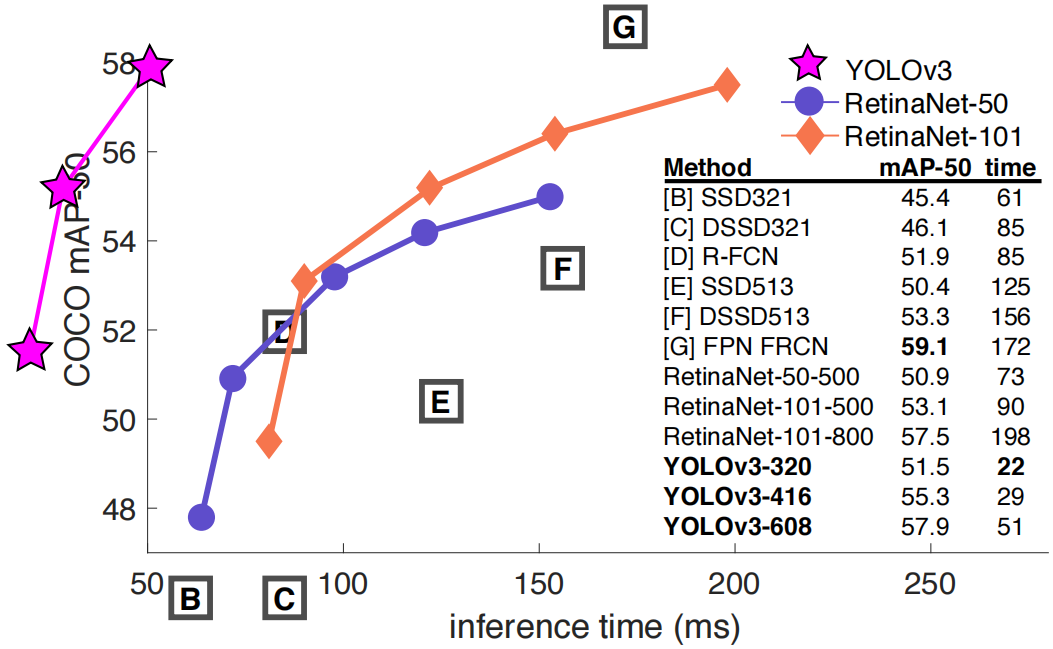
Figure 3. Adapted again from [9], this time showing the speed/accuracy tradeoff on the mAP of the .5 IOU metric. You can tell that YOLOv3 is good because it's tall and far to the left. Can you cite your own paper? Guess who's going to try it, this guy → [16]. Oh, I forgot, we also fixed a data loading bug in YOLOv2, with the help of 2mAP. Just sneaking this here so as not to mess up the layout.
Dual IOU threshold and ground truth assignment. Faster R-CNN uses two IOU thresholds in training. If a prediction overlaps the ground truth by .7, it is a positive example, by [.3−.7] it is ignored, and for all ground truth targets it is less than .3, it is a negative example of. We tried a similar strategy with no good results.
We really like our current formulation, which seems to be at least locally optimal. Some of these techniques may end up yielding good results, perhaps they just need some tweaking to stabilize training.
5. What it all means
YOLOv3 is a good detector. It's fast and accurate. On COCO the average AP is between .5 and .95 IOU metrics, it's not that good. But it is very good on the old detection metric of .5 IOU.
Why do we switch metrics? COCO's original paper has this cryptic line: "Once the evaluation server is complete, a full discussion of the evaluation metrics will be added". Russakovsky et al. report that humans have difficulty distinguishing between 0.3 and .5 IOUs! "It is surprisingly difficult to train a human to visually inspect a bounding box with an IOU of 0.3 and distinguish it from a bounding box with an IOU of 0.5." [18] How difficult is it if humans have difficulty telling the difference? important?
But maybe a better question is: "Now that we have these detectors, what do we do?" A lot of the people doing this research are at Google and Facebook. I think at least we know that the technology is well-handled and certainly not being used to take your personal information and sell it to... wait, you're saying that's exactly what it's for? ? oh
Other people who heavily fund vision research are the military, they've never done anything as horrible as killing a lot of people with new technology oh wait... (Author funded by Office of Naval Research and Google)
I very much hope that most people who use computer vision are just doing some happy good thing with it, like counting zebras in a national park [13], or tracking a cat when it roams the house [19]. But the use of computer vision has been called into question, and it is our responsibility as researchers to at least consider the harm our work may cause and find ways to mitigate it. We owe the world so much.
Finally, don't @ me. (because I finally quit Twitter).
References
[1] Analogy. Wikipedia, Mar 2018. 1
[2] M. Everingham, L. Van Gool, C. K. Williams, J. Winn, and A. Zisserman. The pascal visual object classes (voc) challenge. International journal of computer vision, 88(2):303–338, 2010. 6
[3] C.-Y. Fu, W. Liu, A. Ranga, A. Tyagi, and A. C. Berg. Dssd: Deconvolutional single shot detector. arXiv preprint arXiv:1701.06659, 2017. 3
[4] D. Gordon, A. Kembhavi, M. Rastegari, J. Redmon, D. Fox, and A. Farhadi. Iqa: Visual question answering in interactive environments. arXiv preprint arXiv:1712.03316, 2017. 1
[5] K. He, X. Zhang, S. Ren, and J. Sun. Deep residual learning for image recognition. In Proceedings of the IEEE conference on computer vision and pattern recognition, pages 770–778, 2016. 3
[6] J. Huang, V. Rathod, C. Sun, M. Zhu, A. Korattikara, A. Fathi, I. Fischer, Z. Wojna, Y. Song, S. Guadarrama, et al. Speed/accuracy trade-offs for modern convolutional object detectors. 3
[7] I. Krasin, T. Duerig, N. Alldrin, V. Ferrari, S. Abu-El-Haija, A. Kuznetsova, H. Rom, J. Uijlings, S. Popov, A. Veit, S. Belongie, V. Gomes, A. Gupta, C. Sun, G. Chechik, D. Cai, Z. Feng, D. Narayanan, and K. Murphy. Open-images: A public dataset for large-scale multi-label and multi-class image classification. Dataset available from https://github.com/openimages, 2017. 2
[8] T.-Y. Lin, P. Dollar, R. Girshick, K. He, B. Hariharan, and S. Belongie. Feature pyramid networks for object detection. In Proceedings of the IEEE Conference on Computer Vision and Pattern Recognition, pages 2117–2125, 2017. 2, 3
[9] T.-Y. Lin, P. Goyal, R. Girshick, K. He, and P. Doll´ar. Focal loss for dense object detection. arXiv preprint arXiv:1708.02002, 2017. 1, 3, 4
[10] T.-Y. Lin, M. Maire, S. Belongie, J. Hays, P. Perona, D. Ramanan, P. Doll´ar, and C. L. Zitnick. Microsoft coco: Common objects in context. In European conference on computer vision, pages 740–755. Springer, 2014. 2
[11] W. Liu, D. Anguelov, D. Erhan, C. Szegedy, S. Reed, C.-Y. Fu, and A. C. Berg. Ssd: Single shot multibox detector. In European conference on computer vision, pages 21–37. Springer, 2016. 3
[12] I. Newton. Philosophiae naturalis principia mathematica. William Dawson & Sons Ltd., London, 1687. 1
[13] J. Parham, J. Crall, C. Stewart, T. Berger-Wolf, and D. Rubenstein. Animal population censusing at scale with citizen science and photographic identification. 2017. 4
[14] J. Redmon. Darknet: Open source neural networks in c. http://pjreddie.com/darknet/, 2013–2016. 3
[15] J. Redmon and A. Farhadi. Yolo9000: Better, faster, stronger. In Computer Vision and Pattern Recognition (CVPR), 2017 IEEE Conference on, pages 6517–6525. IEEE, 2017. 1, 2, 3
[16] J. Redmon and A. Farhadi. Yolov3: An incremental improvement. arXiv, 2018. 4
[17] S. Ren, K. He, R. Girshick, and J. Sun. Faster r-cnn: Towards real-time object detection with region proposal networks. arXiv preprint arXiv:1506.01497, 2015. 2
[18] O. Russakovsky, L.-J. Li, and L. Fei-Fei. Best of both worlds: human-machine collaboration for object annotation. In Proceedings of the IEEE Conference on Computer Vision and Pattern Recognition, pages 2121–2131, 2015. 4
[19] M. Scott. Smart camera gimbal bot scanlime:027, Dec 2017. 4
[20] A. Shrivastava, R. Sukthankar, J. Malik, and A. Gupta. Beyond skip connections: Top-down modulation for object detection. arXiv preprint arXiv:1612.06851, 2016. 3
[21] C. Szegedy, S. Ioffe, V. Vanhoucke, and A. A. Alemi. Inception-v4, inception-resnet and the impact of residual connections on learning. 2017. 3