Article directory
Original Link: Address
Personal notes:
Newton (Newton) method, Gauss-Newton (GaussNewton) method, Levenberg-Marquardt (LM) algorithm, etc. Combined with the purpose of realizing the function, the following mainly gives the derivation results, code implementation and some practical applications. At the end of the derivation process, some articles and materials for personal reference will be placed.
One: Newton's method
1 Overview
Newton's method is a function approximation method, its basic idea is: use x ( k ) x^{(k)} near the minimum pointx( k ) second-order Taylor polynomials to approximate the objective functionf ( x ) f(x)f ( x ) , and substitute pointx ( k ) x^{(k)}x( k ) points to the direction of the minimum point of the approximate quadratic function as the search directionp ( k ) p^{(k)}p( k ) .
Suppose a planning problem:minf ( x ) , x ∈ R n min f(x),x∈R^nminf(x),x∈Rn
wheref ( x ) f(x)f ( x ) at pointx ( k ) x^{(k)}x( k ) has a second-order continuous partial derivative, the Hessian matrix▽ 2 f ( x ( k ) ) ▽^2f(x^{(k)})▽2f(x( k ) )is positive definite.
Nowf ( x ) f(x)The kkthminimum point of f ( x )K -level estimated valuex ( k ) x^{(k)}x( k ) , andf ( x ) f(x)f ( x ) as a second-order Taylor expansion:
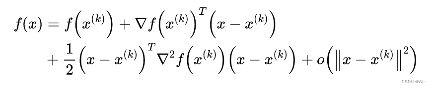 the main ones are the first three items, and the last item is a high-order infinitesimal.
2: Newton's direction and Newton's method
The main parts in the above formula are:

at x ( k ) x^{(k)}x( k ) nearby availableQ ( x ) Q(x)Q ( x ) to approximatef ( x ) f(x)f(x), Q ( x ) ≈ f ( x ) Q(x) ≈ f(x) Q(x)≈f ( x ) .
So we can useQ ( x ) Q(x)The minimum point of Q ( x ) to approximate f ( x ) f(x)The minimum point of f ( x ) , findQ ( x ) Q(x)The stagnation point of Q ( x ) :
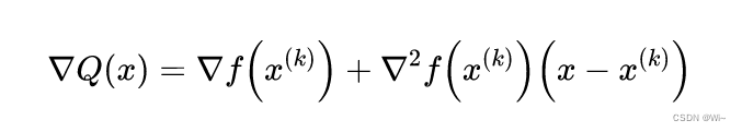
By gradient ▽ Q ( x ) = 0 ▽ Q(x) = 0▽Q(x)=0 getsQ ( x ) Q(x)Stationary pointx ( k + 1 ) x^{(k+1)} of Q ( x )x(k+1), p ( k ) p^{(k)} p( k ) is Newton direction, step sizeλ k \lambda _klkfor 1 11
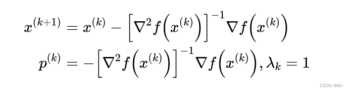
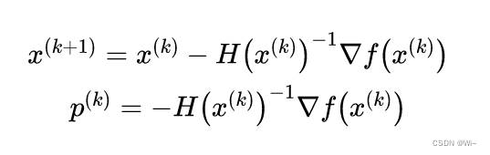
That is described below, where HHH is the Hessian matrix
3: Basic steps of Newton's method
1: Select initial data: initial point x ( 0 ) x^{(0)}x( 0 ) , the termination conditionε > 0 ε>0e>0 , letk : = 0 k:=0k:=0
2: Find the gradient vector▽ f ( k ) ▽ f^{(k)}▽f( k ) , and calculate∣ ∣ ▽ f ( k ) ∣ ∣ ||▽f^{(k)}||∣∣▽f(k)∣∣:
若 ∣ ∣ ▽ f ( k ) ∣ ∣ < ε ||▽f^{(k)}||<ε ∣∣▽f(k)∣∣<ε , stop selection, outputx ( k ) x^{(k)}x( k ) , otherwise go to the next step.
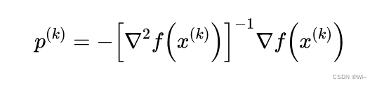
3: Construct Newton direction:
4: Algorithm iteration:
Solution x ( k + 1 ) = x ( k ) + p ( k ) x^{(k+1)} = x^{(k)} + p^{(k)}x(k+1)=x(k)+p( k ) withx ( k + 1 ) x^{(k+1)}x( k + 1 ) as the next iteration point, letk : = k + 1 k := k+1k:=k+1 , turn to step 2.
4: Example
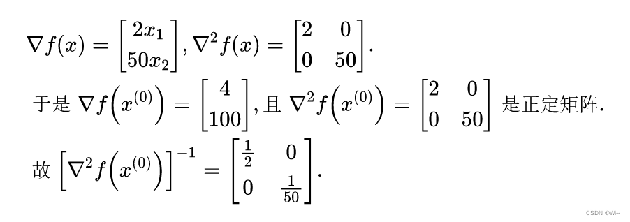
Use Newton's method to find the function f ( x ) = x 1 2 + 25 x 2 2 f(x) = x_1^2 + 25x_2^2f(x)=x12+25x22, where the initial point is x ( 0 ) = ( 2 , 2 ) T x^{(0)} = (2, 2)^Tx(0)=(2,2)T ,ε = 1 0 − 6 ε = 10^{-6}e=10− 6. Solution
(1) Find the gradient and Hessian matrix:
(2) Determine Newton's direction:
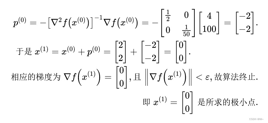 namely: x 1 = 0 , x 2 = 0 x_1 = 0, x_2=0x1=0,x2=0
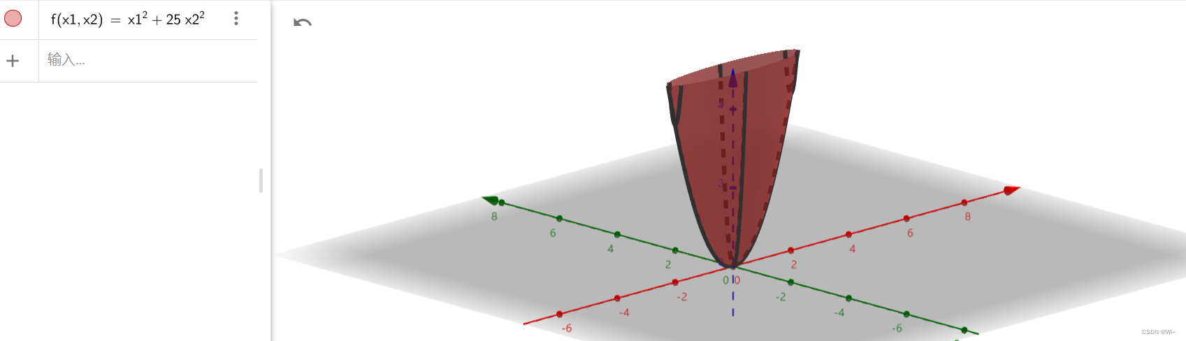
Here the three-dimensional coordinate system is used to view x 1 = 0 , x 2 = 0 x_1 = 0, x_2=0x1=0,x2=There is an extreme value at 0
Here, the Newton method has a disadvantage of using the Hessian matrix: the amount of calculation is particularly large. The Gauss-Newton method is introduced below, which replaces the Hessian matrix with the Jacobian matrix on the basis of the Newton method.
Two: Gauss–Newton algorithm (Gauss–Newton algorithm)
1 Overview
The Gauss-Newton algorithm is used to solve nonlinear least squares problems, which is equivalent to minimizing the sum of squares of function values. It is an extension of Newton's method of finding the minimum value of a nonlinear function. Since the sum of squares must be non-negative, the algorithm can be viewed as using Newton's method to iteratively approximate the zero of the sum, thereby minimizing the sum. It has the advantage of not needing to compute the potentially challenging second derivative (aka the Hessian matrix).
Note: The Gauss-Newton method is for nonlinear least squares problems. Detailed Least Squares
2: Gauss-Newton method derivation
①: Objective function problem: independent variable xxx obtains the dependent variableyyy, m m m observation points:
X = [ x 1 , x 2 , . . . xm ] TX=[x_1,x_2,...x_m]^TX=[x1,x2,...xm]T, Y = [ y 1 , y 2 , . . . y m ] T Y=[y_1,y_2,...y_m]^T Y=[y1,y2,...ym]T
②:model function:Y = f ( X ; β 1 , β 2 , . . . , β n ) Y = f(X;β_1,β_2,...,β_n)Y=f(X;b1,b2,...,bn) =>f ( x ; β ) f(x; β)f(x;b )
where xxx is the independent variable,yyy is the dependent variable,β ββ is the target parameter. x and yx and yx and y are known, optimizeβ ββ target parameter.
③:Preference index function: min S = ∑ i = 1 n ( f ( xi ; β ) − yi ) 2 min S = \displaystyle\sum_{i=1}^{n}(f(x_i;β)-y_i )^2minS=i=1∑n(f(xi;b )−yi)2
④: No.iiPrediction deviation of observation point i : ri = f ( xi ; β ) − yi ) 2 r_i = f(x_i;β)-y_i)^2ri=f(xi;b )−yi)2 , then each deviation forms a vector form:R = [ r 1 , r 2 , . . . rm ] TR = [r_1,r_2,...r_m]^TR=[r1,r2,...rm]T
⑤: For ③ objective function can be written as:min S = ∑ i = 1 nri 2 = RTR min S = \displaystyle\sum_{i=1}^{n}r_i^2 = R^TRminS=i=1∑nri2=RT R
⑥: 是电影电视支度:▽ S ( β ) = [ ∂ S ∂ β 1 , ∂ S ∂ β 2 , . . . , ∂ S ∂ β n ] T ▽S(β) = [\frac{\partial S}{\partial β_1},\frac{\partial S}{\partial β_2},...,\frac{\partial S}{\partial β_n}]^T▽ S ( b )=[∂β1∂S,∂β2∂S,...,∂βn∂S]T , where for each parameterβ j β_jbj求偏密∂ S ∂ β j = 2 ∑ i = 1 mri ∂ ri ∂ β j \frac{\partial S}{\partial β_j} = 2 \displaystyle\sum_{i=1}^{m}r_i\frac {\partial r_i}{\partial β_j}∂βj∂S=2i=1∑mri∂βj∂ri
⑦: For R = [ r 1 , r 2 , . . . rm ] T and β R = [r_1,r_2,...r_m]^T and βR=[r1,r2,...rm]The partial derivatives of T andβcan be written as the Jacobian matrix
J ( R ( β ) ) = [ ∂ r 1 ∂ β 1 . . . ∂ r 1 ∂ β n ⋮ ⋱ ⋮ ∂ rm ∂ β 1 . . . ∂ rm ∂ β n ] J(R(β)) = \begin{bmatrix} \frac{\partial r_1}{\partial β_1}&...&\frac{\partial r_1}{\partial β_n}\\ \vdots & \ddots & \vdots \\ \frac{\partial r_m}{\partial β_1}&...&\frac{\partial r_m}{\partial β_n}\end{bmatrix}J(R(β))= ∂β1∂r1⋮∂β1∂rm...⋱...∂βn∂r1⋮∂βn∂rm
⑧:target function 梢度(一駖偏寛):▽ S ( β ) = [ ∂ S ∂ β 1 , ∂ S ∂ β 2 , . . . , ∂ S ∂ β n ] T = > ∂ S ∂ β j = 2 ∑ i = 1 mri ∂ ri ∂ β j = > ▽ S = 2 JTR ▽S(β) = [\frac{\partial S}{\ partial β_1},\frac{\partial S}{\partial β_2},...,\frac{\partial S}{\partial β_n}]^T => \frac{\partial S}{\partial β_j} = 2 \displaystyle\sum_{i=1}^{m}r_i\frac{\partial r_i}{\partial β_j} => ▽S = 2J^TR▽ S ( b )=[∂β1∂S,∂β2∂S,...,∂βn∂S]T=>∂βj∂S=2i=1∑mri∂βj∂ri=>▽S=2 JT R
⑨: Find the objective function Hessian matrix (second-order partial derivative):
from the gradient vector element∂ S ∂ β j = 2 ∑ i = 1 mri ∂ ri ∂ β j \frac{\partial S}{\partial β_j} = 2 \displaystyle\sum_{i=1}^{m}r_i\frac{\partial r_i}{\partial β_j}∂βj∂S=2i=1∑mri∂βj∂ri到黑塞ボタッシット∂ 2 S ∂ β k ∂ β j = 2 ∂ ∂ β k ( ∑ i = 1 mri ∂ ri ∂ β j ) \frac{\partial ^2S}{\partial β_k\partial β_j} = 2 \frac{\partial }{\partial β_k} (\displaystyle\sum_{i=1}^{m}r_i\frac{\partial r_i}{\partial β_j})∂βk∂βj∂2S=2∂βk∂(i=1∑mri∂βj∂ri),
applicability of chain式法则得:∂ 2 S ∂ β k ∂ β j = 2 ∑ i = 1 m ( ∂ ri ∂ β k ∂ ri ∂ β j + ri ∂ 2 ri ∂ β k ∂ β j ) \frac{ \partial ^2S}{\partial β_k\partial β_j} = 2 \displaystyle\sum_{i=1}^{m}(\frac{\partial r_i}{\partial β_k}\frac{\partial r_i}{\ partial β_j} + r_i\frac{\partial^2 r_i}{\partial β_k\partial β_j})∂βk∂βj∂2S=2i=1∑m(∂βk∂ri∂βj∂ri+ri∂βk∂βj∂2 ri) ,
among whichOOO matrix element :O kj = ∑ i = 1 mri ∂ 2 ri ∂ β k ∂ β j O_{kj} = \displaystyle\sum_{i=1}^{m}r_i\frac{\partial^2 r_i}{ \partial β_k\partial β_j}Okj=i=1∑mri∂βk∂βj∂2 ri
Hessian matrix: H = 2 ( JTJ + O ) H = 2(J^TJ + O)H=2(JTJ+O )
⑩: Written in the form of Newton's method: if the model is better, whereOOO squareri r_iriis close to 0. OO _The O matrix is ignored for the convenience of calculation.
3: Gauss-Newton method algorithm flow
1: given initial parameter value β 0 β_0b0(default is 1 11 vector). Letε = 1 − 10 ε = 1^{-10}e=1− 10
2: For thekkthK times selection, find the current Jacobian matrixJ ( β k ) J(β_k)J ( bk) and residual valuef ( β k ) f(β_k)f ( bk) isRRR. _
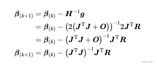
3: Solve the incremental equation:H Δ β k = − g H\Delta β_k = -gH D bk=− g
=> Δ β k = − H − 1 g \Delta β_k= -H^{-1}gD bk=−H−1g
=> Δ β k ≈ − ( J T J ) − 1 J T R \Delta β_k≈ -(J^TJ)^{-1}J^TR D bk≈−(JTJ)- 1 JT R. Here the Jacobian matrixJTJJ^TJJT JApproximate Hessian MatrixHHH。
4:若Δ β k < ε \Delta β_k<εD bk<ε,则最作。 otherwise,令β k + 1 = β k + Δ β k β_{k+1} = β_k +\Delta β_kbk+1=bk+D bk, return to step 2.
4: Gauss-Newton method C++ code
   /* 高斯牛顿法(GNA) 解决非线性最小二乘问题 确定目标函数和约束来对现有的参数优化
     */

    template <class _T,class _ResidualsVector,class _JacobiMat>
    Eigen::VectorXd GaussNewtonAlgorithm(Eigen::VectorXd params,_T otherArgs, _ResidualsVector ResidualsVector,_JacobiMat JacobiMat,double _epsilon = 1e-10,int _maxIteCount = 999)
    {


        int k=0;
        // ε 终止条件
        double epsilon = _epsilon;
        //迭代次数
        int maxIteCount = _maxIteCount;

        //found 为true 结束循环
        bool found = false;
        while(!found && k<maxIteCount)
        {


            //迭代增加
            k++;
            //获取预测偏差值 r= ^y(预测值) - y(实际值)
            //保存残差值
            Eigen::VectorXd residual = ResidualsVector(params,otherArgs);

            //求雅可比矩阵
            Eigen::MatrixXd Jac = JacobiMat(params,otherArgs);

            // Δx = - (Jac^T * Jac)^-1 * Jac^T * r
            Eigen::VectorXd delta_x =  -  (((Jac .transpose() * Jac ).inverse()) * Jac.transpose() * residual).array();

            qDebug()<<QString("高斯牛顿法:第 %1 次迭代 --- 精度:%2  ").arg(k).arg(delta_x.array().abs().sum());
            //达到精度,结束
            if(delta_x.array().abs().sum() < epsilon)
            {


                found = true;
            }

            //x(k+1) = x(k) + Δx
            params = params + delta_x;

        }
        return params;
    }
Matrix is a matrix class in the Eigen library , and the Eigen library is introduced here to facilitate algebraic operations.
Approximate Hessian matrix J ( x ) TJ ( x ) J(x)^TJ(x)J(x)T J(x)may be a singular matrix or ill-conditioned, the following leads toLM LMLM algorithm .
Three: Levenberg-Marquardt algorithm (Levenberg-Marquardt algorithm)
1 Overview
In mathematics and computing, the Levenberg–Marquardt algorithm (LMA or simply LM), also known as the damped least squares method (DLS), is used to solve nonlinear least squares problems. These minimization problems arise especially in least squares curve fitting. LMA interpolates between Gauss-Newton Algorithm (GNA) and Gradient Descent. LMA is more robust than GNA, which means that in many cases it can find a solution even if it starts off far from the final minimum. For well-behaved functions and reasonable startup parameters, LMA tends to be slower than GNA. LMA can also be viewed as a Gauss-Newton using a trust region approach.
LMA is used in many software applications to solve general curve fitting problems. By using the Gauss-Newton algorithm, it usually converges faster than first-order methods. However, like other iterative optimization algorithms, LMA can only find local minima, not necessarily global minima. Like other numerical minimization algorithms, the Levenberg–Marquardt algorithm is an iterative process. To start the minimization, the user must provide an initial guess β for the parameter vector ββ , where there is only one minimum, an uninformed standard guess would be something likeβ = [ 1 , 1 , . . . , 1 ] T β = [1,1,...,1]^Tb=[1,1,...,1]T will work just fine; in the case of multiple minima, the algorithm will only converge to the global minimum when the initial guess is already somewhat close to the final solution.
2: LM algorithm process
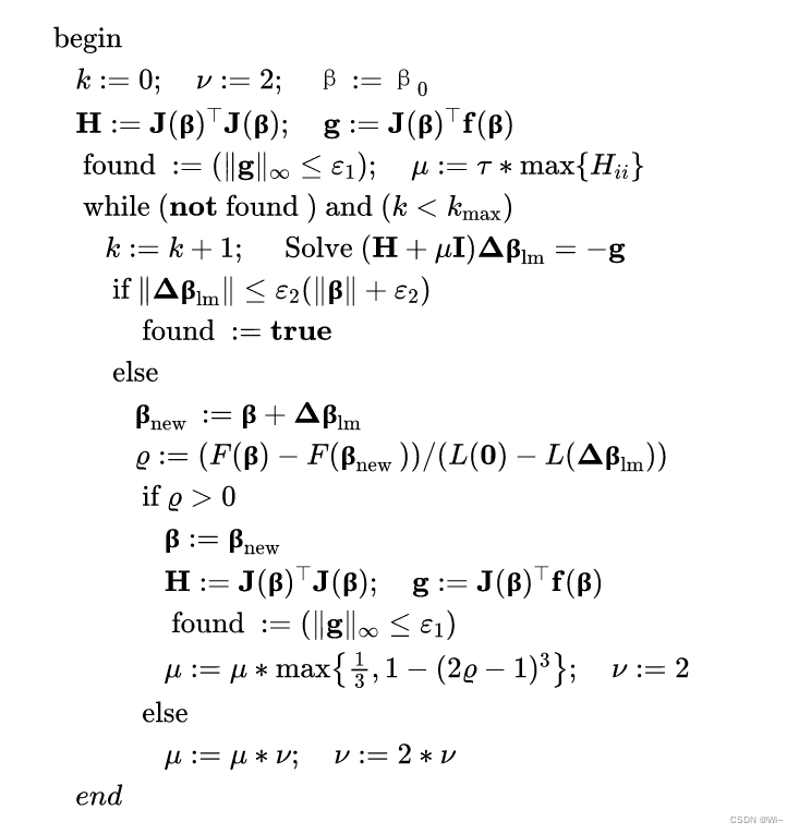
1: given initial parameter value β 0 β_0b0(default is 1 11 vector). initialμ 0 μ_0m0The choice of can depend on H 0 = J ( β 0 ) TJ ( β 0 ) H_0=J(β_0)^TJ(β_0)H0=J ( b0)T J(β0) , generally we chooseμ 0 = τ ∗ maxi { H ii ( 0 ) } μ_0 =τ*max_i\{H_{ii}^{(0)}\}m0=t∗maxi{ Hii(0)},generalτ= 1 0 − 6 τ=10^{−6}t=10− 6 , here we setε 1 = 1 − 10 ε_1 = 1^{-10}e1=1− 10和ε 2 = 1 − 10 ε_2 = 1^{-10}e2=1−10 . _
2: If∣ ∣ g ∣ ∣ ∞ ≤ ε 1 ||g||_\infty≤ε_1∣∣g∣∣∞≤e1established, stop.
3: For the kthK times selection, find the current Jacobian matrixJ ( β k ) J(β_k)J ( bk) and residual valuef ( β k ) f(β_k)f ( bk) isRRR. _
4: Solve the incremental equation:( H + μ k I ) Δ β k = − g (H+μ_kI)\Delta β_k = -g(H+mkI ) D bk=− g
=> Δ β k = − ( H + μ k I ) − 1 g \Delta β_k= -(H+μ_kI)^{-1}gD bk=−(H+mkI)−1g
=> Δ β k ≈ − ( J T J + μ k I ) − 1 J T R \Delta β_k≈ -(J^TJ+μ_kI)^{-1}J^TR D bk≈−(JTJ+mkI)- 1 JT R. Here the Jacobian matrixJTJJ^TJJT JApproximate Hessian MatrixHHH。
5:若∣ ∣ Δ β k ∣ ∣ ≤ ε 2 ( ∣ ∣ β k ∣ ∣ + ε 2 ) ||\Delta β_k||≤ε_2(||β_k|| + ε_2)∣∣Δβk∣∣≤e2(∣∣βk∣∣+e2) is established, then stop. Otherwise, letβ k + 1 = β k + Δ β k β_{k+1} = β_k +\Delta β_kbk+1=bk+D bk。
6:ρ = ∣ ∣ F ( β k ) ∣ ∣ 2 2 − ∣ ∣ F ( β k + Δ β k ) ∣ ∣ 2 2 L ( 0 ) − L ( Δ β k ) \rho = \frac{| |F(β_k)||_2^2-||F(β_k+\Delta β_k)||_2^2}{L(0) - L(\Delta β_k)}r=L ( 0 ) − L ( Δ bk)∣∣ F ( bk)∣∣22− ∣∣ F ( bk+ D bk)∣∣22, if ρ > 0 \rho >0r>0 , find the current Hessian matrixH ≈ J ( β k ) TJ ( β k ) H ≈ J(β_k)^TJ(β_k)H≈J ( bk)T J(βk) and gradientg = J ( β k ) T f ( β k ) g = J(β_k)^Tf(β_k)g=J ( bk)Tf(βk) . If∣ ∣ g ∣ ∣ ∞ ≤ ε 1 ||g||_\infty≤ε_1∣∣g∣∣∞≤e1established, stop. Update μ k μ_kmk,μ k = μ k ∗ max { 1 3 , 1 − ( 2 ρ − 1 ) 3 } ; v = 2 μ_k =μ_k*max\{\frac{1}{3},1-(2\rho-1)^3\};v=2mk=mk∗max{ 31,1−( 2 p−1)3};v=2 . Ifρ ≤ 0 \rho ≤ 0r≤0,μ k = μ k ∗ v ; v = 2 ∗ v μ_k =μ_k*v; v=2*vmk=mk∗v;v=2∗v。
The final pseudocode is as follows:
3: Levenberg-Marquardt method C++ code
/* 列文伯格马夸尔特法(LMA) == 使用信赖域的高斯牛顿法,鲁棒性更好, 确定目标函数和约束来对现有的参数优化
* params 初始参数,待优化
* otherArgs 其他参数
* _ResidualsVector 自定义函数:获取预测值和实际值的差值
* _JacobiMat 自定义函数:获取当前的雅可比矩阵
* _epsilon 收敛精度
* _maxIteCount 最大迭代次数
* _epsilon 和 _maxIteCount 达到任意一个条件就停止返回
*/
template <class _T,class _ResidualsVector,class _JacobiMat>
Eigen::VectorXd LevenbergMarquardtAlgorithm(Eigen::VectorXd ¶ms,_T otherArgs, _ResidualsVector ResidualsVector,_JacobiMat JacobiMat,double _epsilon = 1e-12,quint32 _maxIteCount = 99)
{
quint32 iterCount=0;
double currentEpsilon =0.;
QElapsedTimer eTimer;
// ε 终止条件
double epsilon = _epsilon;
double _currentEpsilon=0.0;
// τ
double tau = 1e-6;
//迭代次数
quint32 maxIteCount = _maxIteCount;
quint32 k=0;
int v=2;
//求雅可比矩阵
Eigen::MatrixXd Jac = JacobiMat(params,otherArgs);
//用雅可比矩阵近似黑森矩阵
Eigen::MatrixXd Hessen = Jac .transpose() * Jac ;
//获取预测偏差值 r= ^y(预测值) - y(实际值)
//保存残差值
Eigen::VectorXd residual = ResidualsVector(params,otherArgs);
//梯度
Eigen::MatrixXd g = Jac.transpose() * residual;
//found 为true 结束循环
bool found = ( g.lpNorm<Eigen::Infinity>() <= epsilon );
//阻尼参数μ
double mu = tau * Hessen.diagonal().maxCoeff();
eTimer.restart();
while(!found && k<maxIteCount)
{
k++;
//LM方向 uI => I 用黑森矩阵对角线代替
//Eigen::MatrixXd delta_x = - (Hessen + mu*Hessen.asDiagonal().diagonal()).inverse() * g;
Eigen::VectorXd delta_x = - (Hessen + mu*Eigen::MatrixXd::Identity(Hessen.cols(), Hessen.cols())).inverse() * g;
if( delta_x.lpNorm<2>() <= epsilon * (params.lpNorm<2>() + epsilon ))
{
currentEpsilon = delta_x.lpNorm<2>();
found = true;
}
else
{
Eigen::VectorXd newParams = params + delta_x;
//L(0) - L(delta) = 0.5*(delta^-1)*(μ*delta - g)
//ρ = (F(x) - F(x_new)) / (L(0) - L(delta));
double rho = (ResidualsVector(params,otherArgs).array().pow(2).sum() - ResidualsVector(newParams,otherArgs).array().pow(2).sum())
/ (0.5*delta_x.transpose()*(mu * delta_x - g)).sum();
if(rho>0)
{
params = newParams;
Jac = JacobiMat(params,otherArgs);
Hessen = Jac.transpose() * Jac ;
//获取预测偏差值 r= ^y(预测值) - y(实际值)
residual = ResidualsVector(params,otherArgs);
g = Jac.transpose() * residual;
_currentEpsilon = g.lpNorm<Eigen::Infinity>();
found = (_currentEpsilon <= epsilon );
mu = mu* qMax(1/3.0 , 1-qPow(2*rho -1,3));
v=2;
}
else
{
mu = mu*v;
v = 2*v;
}
}
iterCount=k;
currentEpsilon = _currentEpsilon;
//发送 当前迭代次数,当前精度,迭代一次需要的时长
qDebug()<<QString("当前迭代次数: %1 ,收敛精度: %2 ,迭代时长: %3 ").arg(iterCount).arg(currentEpsilon).arg(eTimer.restart());
}
return params;
}
//====================================================================
//====================================================================
// 例子:下面是曲线拟合使用lm算法来优化,残差值向量和雅可比矩阵需要自己编写
#define DERIV_STEP 1e-5
//线拟合残差值向量
class LineFitResidualsVector
{
public:
Eigen::VectorXd operator()(const Eigen::VectorXd& parameter,const QList<Eigen::MatrixXd> &otherArgs)
{
Eigen::MatrixXd inValue = otherArgs.at(0);
Eigen::VectorXd outValue = otherArgs.at(1);
int dataCount = inValue.rows();
int paramsCount = parameter.rows();
//保存残差值
Eigen::VectorXd residual = Eigen::VectorXd::Zero(dataCount);
//获取预测偏差值 r= ^y(预测值) - y(实际值)
for(int i=0;i<dataCount;++i)
{
for(int j=0;j<paramsCount;++j)
{
//这里使用曲线方程 y = a1*x^0 + a2*x^1 + a3*x^2 + ... 根据参数(a1,a2,a3,...)个数来设置
residual(i) += parameter(j) * inValue(i,j);
}
}
return residual - outValue;
}
};
//求线拟合雅克比矩阵 -- 通过计算求偏导
class LineFitJacobi
{
//求偏导
double PartialDeriv(const Eigen::VectorXd& parameter,int paraIndex,const Eigen::MatrixXd &inValue,int objIndex)
{
Eigen::VectorXd para1 = parameter;
Eigen::VectorXd para2 = parameter;
para1(paraIndex) -= DERIV_STEP;
para2(paraIndex) += DERIV_STEP;
//逻辑
double obj1 = 0;
double obj2 = 0;
for(int i=0;i<parameter.rows();++i)
{
//这里使用曲线方程 y = a1*x^0 + a2*x^1 + a3*x^2 + ... 根据参数(a1,a2,a3,...)个数来设置
obj1 += para1(i) * inValue(objIndex,i);
}
for(int i=0;i<parameter.rows();++i)
{
//这里使用曲线方程 y = a1*x^0 + a2*x^1 + a3*x^2 + ... 根据参数(a1,a2,a3,...)个数来设置
obj2 += para2(i) * inValue(objIndex,i);
}
return (obj2 - obj1) / (2 * DERIV_STEP);
}
public:
Eigen::MatrixXd operator()(const Eigen::VectorXd& parameter,const QList<Eigen::MatrixXd> &otherArgs)
{
Eigen::MatrixXd inValue = otherArgs.at(0);
int rowNum = inValue.rows();
int paramsCount = parameter.rows();
Eigen::MatrixXd Jac(rowNum, paramsCount);
for (int i = 0; i < rowNum; i++)
{
for (int j = 0; j < paramsCount; j++)
{
Jac(i,j) = PartialDeriv(parameter,j,inValue,i);
}
}
return Jac;
}
};
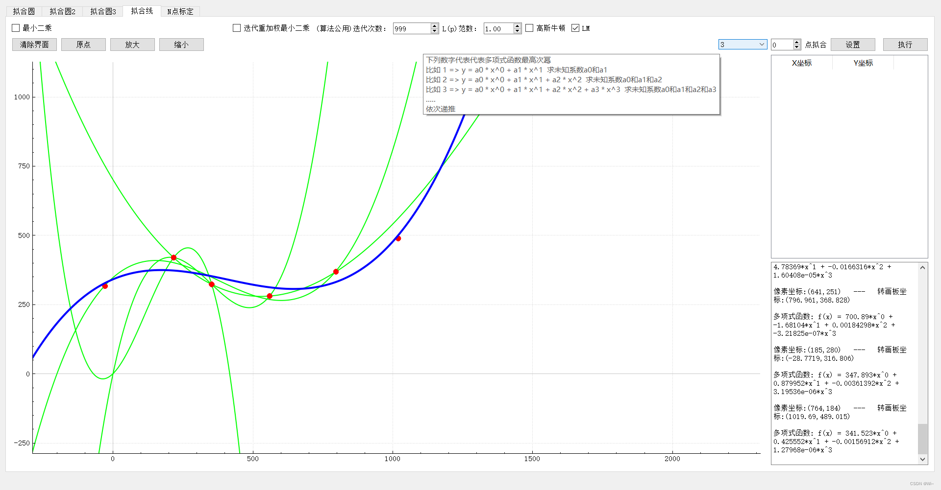
/* y = a0 * x^0 + a1 * x^1 求未知系数a0和a1\n"
* y = a0 * x^0 + a1 * x^1 + a2 * x^2 求未知系数a0和a1和a2\n"
* y = a0 * x^0 + a1 * x^1 + a2 * x^2 + a3 * x^3 求未知系数a0和a1和a2和a3\n"
*
* 矩阵描述
* _ _ _ _ _ _
* |1 x1 x1^2 ...| | a0 | |y1 |
* |1 x2 x2^2 ...| | a1 | =|y2 |
* |1 x3 x3^2 ...| | a2 | |y3 |
* |1 x4 x4^2 ...| | .. | |y4 |
* |.... ...| - - |...|
* - - - -
* Ax = B
*/
QList<double> coeffL;
//数据个数
int rows = listP.count();
int col = m_maxPower + 1;
//m_maxPower
VectorXd vector_x;
//创建动态n行,3列矩阵
MatrixXd matA;
matA.resize(rows,col);
VectorXd matB;
matB.resize(rows,1);
//构建矩阵
for(int i=0;i<rows;++i)
{
//A
for(int j=0;j<col;++j)
{
matA(i,j) = std::pow(listP.at(i).x(),j);
}
//B
matB(i,0) = listP.at(i).y();
}
//勾选高斯牛顿法
if(m_GN->isChecked())
{
int iteCount= m_iterationCount->value();
//初始参数为1
VectorXd args = VectorXd::Ones(m_maxPower+1);
QList<MatrixXd> otherArgs;
otherArgs.append(matA);
otherArgs.append(matB);
vector_x =GaussNewtonAlgorithm(args,otherArgs,LineFitResidualsVector(),LineFitJacobi(),1e-10,iteCount);
}
//勾选LM
else if(m_LM->isChecked())
{
int iteCount= m_iterationCount->value();
//初始参数为1
VectorXd args = VectorXd::Ones(m_maxPower+1);
QList<MatrixXd> otherArgs;
otherArgs.append(matA);
otherArgs.append(matB);
LevenbergMarquardtAlgorithm(args,otherArgs,LineFitResidualsVector(),LineFitJacobi(),1e-15,iteCount);
}
Four: Summary
1: Gauss-Newton method and LM LMThe LM algorithm belongs to the optimal least squares algorithm, and in the case of given initial parameters, the parameters are further optimized, whileLM LMThe LM algorithm has better robustness, but at the expense of a certain convergence speed. (Optimization understanding: In mathematics, optimization in a narrow sense refers to a class of problems. It has three elements: optimization variables, objective functions, and constraints. Under the condition of satisfying the constraints, the optimization variables are adjusted to minimize the value of the objective function. This is The simplest interpretation of the optimization problem). Newton's method is suitable for finding extreme values.
2: Tools: The main Qt +Eigen library
Eigen library is a library for matrix calculations and algebraic calculations
3: The complete code above has been uploaded to GitHub
4: References Hessian
matrix and Jacobian matrix Understanding
Gauss-Newton method Detailed explanation of
LM algorithm Detailed explanation
of LM paper