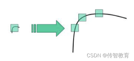
Earlier we introduced the Harris and Shi-Tomasi corner detection algorithms. These two algorithms have rotation invariance, but not scale invariance. Take the following figure as an example. Corners can be detected in the small picture on the left, but the image is After zooming in, using the same window, the corners cannot be detected.
So, let's introduce a computer vision algorithm, scale-invariant feature transform or SIFT (Scale-invariant feature transform). It is used to detect and describe local features in images. It looks for extreme points in the spatial scale and extracts its position, scale, and rotation invariants. This algorithm was published by David Lowe in 1999 and perfected in 2004. Summarize. Applications include object recognition, robot map perception and navigation, image stitching, 3D model building, gesture recognition, image tracking, and motion comparison.
The essence of the SIFT algorithm is to find key points (feature points) in different scale spaces and calculate the direction of the key points. The key points found by SIFT are some very prominent points that will not change due to factors such as illumination, affine transformation and noise, such as corner points, edge points, bright spots in dark areas, and dark points in bright areas.
1.1 Basic process
Lowe decomposes the SIFT algorithm into the following four steps:
Scale-space extrema detection: Searches for image locations at all scales. Potential keypoints that are invariant to scale and rotation are identified by a Gaussian difference function.
Keypoint positioning: At each candidate location, a fine-fitting model is used to determine the location and scale. Keypoints are chosen according to their stability.
Keypoint orientation determination: assign one or more orientations to each keypoint position based on the local gradient orientation of the image. All subsequent operations on the image data are transformed relative to the orientation, scale, and position of the keypoints, thereby ensuring invariance to these transformations.
Keypoint description: In the neighborhood around each keypoint, the local gradient of the image is measured at a selected scale. These gradients serve as keypoint descriptors, which allow relatively large local shape deformations or lighting changes.
Let's follow Lowe's steps to introduce the implementation process of the SIFT algorithm:
1.2 Extremum detection in scale space
It is not possible to use the same window to detect extreme points in different scale spaces, use a small window for small key points, and use a large window for large key points. In order to achieve the above goals, we use scale space filters.
The Gaussian kernel is the only kernel function that can generate a multi-scale space. - "Scale-space theory: A basic tool for analyzing structures at different scales".
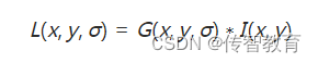
The scale space L(x,y,σ) of an image is defined as the convolution operation of the original image I(x,y) with a variable-scale 2-dimensional Gaussian function G(x,y,σ), namely: where
:
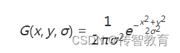
σ is the scale space factor, which determines the degree of blurring of the image. On a large scale (with a large σ value), the general information of the image is represented, and on a small scale (with a small σ value), the detailed information of the image is represented.
When calculating the discrete approximation of the Gaussian function, the pixels outside the approximate 3σ distance can be regarded as ineffective, and the calculation of these pixels can be ignored. Therefore, in practical applications, only calculating the Gaussian convolution kernel of (6σ+1)*(6σ+1) can guarantee the influence of relevant pixels.
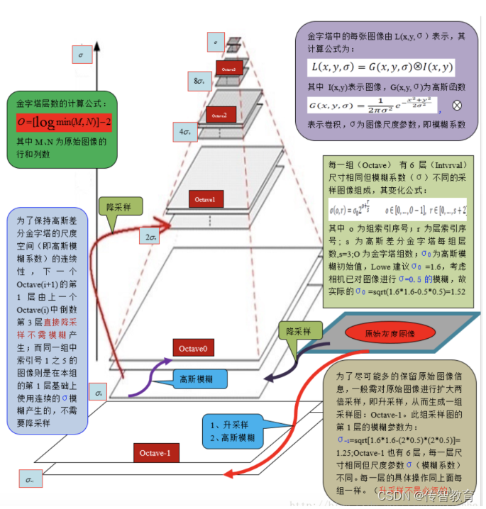
Next, we construct the Gaussian pyramid of the image, which is obtained by blurring and downsampling the image with the Gaussian function. During the construction of the Gaussian pyramid, the image is first doubled, and the Gaussian pyramid is constructed on the basis of the enlarged image, and then the The image under this size is Gaussian blurred, and several blurred images form an Octave, and then select an image under the Octave to downsample, the length and width are doubled, and the image area becomes a quarter of the original . This image is the initial image of the next Octave. On the basis of the initial image, the Gaussian blur processing belonging to this Octave is completed, and so on to complete all the octave constructions required by the entire algorithm, so that the Gaussian pyramid is constructed. The entire The process is shown in the figure below:
Using LoG (Laplacian of Gaussian method), that is, the second derivative of the image, the key point information of the image can be detected at different scales, so as to determine the feature points of the image. However, LoG is computationally intensive and inefficient. So we obtain DoG (difference of Gaussian) to approximate LoG by subtracting images of two adjacent Gaussian scale spaces.
In order to calculate DoG, we build a Gaussian difference pyramid, which is built on the basis of the above-mentioned Gaussian pyramid. The establishment process is: in the Gaussian pyramid, the subtraction of two adjacent layers in each Octave constitutes a Gaussian difference pyramid. As shown below:
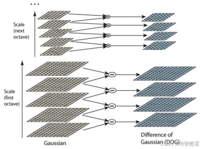
The first group and the first layer of the Gaussian difference pyramid are obtained by subtracting the first group and the first layer from the first group and the second layer of the Gaussian pyramid. By analogy, each difference image is generated group by group and layer by layer, and all difference images form a difference pyramid. It is summarized that the image of the oth group l layer of the DOG pyramid is obtained by subtracting the oth group l layer from the oth group l+1 layer of the Gaussian pyramid. The extraction of subsequent Sift feature points is carried out on the DOG pyramid
After DoG is done, local maxima can be searched in different scale spaces. For a pixel in the image, it needs to be compared with the 8 neighbors around it and the adjacent 18 (2x9) points in the upper and lower layers in the scale space. If it's a local maximum, it might be a key point. Basically the keypoint is the best representation of the image in the corresponding scale space. As shown below:
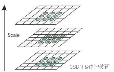
The search process starts from the second layer of each group, takes the second layer as the current layer, and takes a 3×3 cube for each point in the DoG image of the second layer, and the upper and lower layers of the cube are the first layer and the third layer . In this way, the searched extreme points have both position coordinates (DoG image coordinates) and spatial scale coordinates (layer coordinates). After the second layer search is completed, the third layer is used as the current layer, and the process is similar to the second layer search. When S=3, there are 3 layers to be searched in each group, so there are S+2 layers in the DOG, and each group has S+3 layers in the pyramid constructed at the beginning.
1.3 Key point positioning
Since DoG is sensitive to noise and edges, the local extremum points detected in the above Gaussian difference pyramid need further inspection before they can be accurately positioned as feature points.
The exact position of the extremum is obtained by using the Taylor series expansion of the scale space. If the gray value of the extremum point is less than the threshold (usually 0.03 or 0.04), it will be ignored. This threshold is called contrastThreshold in OpenCV.
The DoG algorithm is very sensitive to the boundary, so we have to remove the boundary. In addition to being used for corner detection, the Harris algorithm can also be used for detecting boundaries. From the algorithm of Harris corner detection, when one eigenvalue is much larger than another eigenvalue, it is detected as a boundary. The key points that are not good in the DoG algorithm have a larger main curvature in the direction parallel to the edge, and a smaller curvature in the direction perpendicular to the edge. If the ratio of the two is higher than a certain threshold (called in OpenCV Boundary threshold), the key point is considered to be a boundary and will be ignored. Generally, the threshold is set to 10.
The key points of low contrast and boundaries are removed, and the key points we are interested in are obtained.
1.4 Key point direction determination
After the above two steps, the key points of the image are completely found, and these key points are scale invariant. In order to achieve rotation invariance, it is also necessary to assign a direction angle to each key point, that is, to obtain a direction reference based on the neighborhood structure of the Gaussian scale image where the detected key point is located.
For any key point, we collect the gradient features (magnitude and argument) of all pixels in the Gaussian pyramid image where the radius is r, and the radius r is:
r=3×1.5s
Where σ is the scale of the octave image where the key point is located, and the corresponding scale image can be obtained.
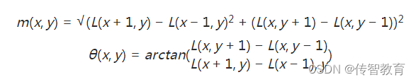
The formulas for calculating the magnitude and direction of the gradient are:
The calculation result of the neighborhood pixel gradient is shown in the figure below:
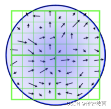
After completing the key point gradient calculation, use the histogram to count the gradient magnitude and direction of the pixels in the key point neighborhood. The specific method is to divide 360° into 36 columns, and every 10° is a column, and then in the area with r as the radius, find the pixels whose gradient direction is in a certain column, and then add their amplitudes together as the height of the column. Because the contribution of the gradient magnitude of the pixel to the central pixel is different in the area where r is the radius, it is also necessary to weight the magnitude, using Gaussian weighting with a variance of 1.5σ. As shown in the figure below, only the histograms in 8 directions are drawn in order to simplify the figure.
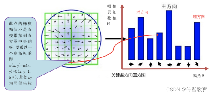
Each feature point must be assigned a main direction, and one or more auxiliary directions are required. The purpose of adding auxiliary directions is to enhance the robustness of image matching. The definition of the auxiliary direction is that when the height of a cylinder is greater than 80% of the height of the main direction cylinder, the direction represented by the cylinder is the auxiliary direction for the feature point.
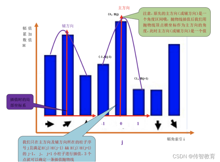
The peak value of the histogram, that is, the direction represented by the highest column is the main direction of the image gradient within the neighborhood of the feature point, but the angle represented by the column is a range, so we need to interpolate and fit the discrete histogram, In order to get a more accurate direction angle value. Use a parabola to fit the discrete histogram, as shown in the following figure:
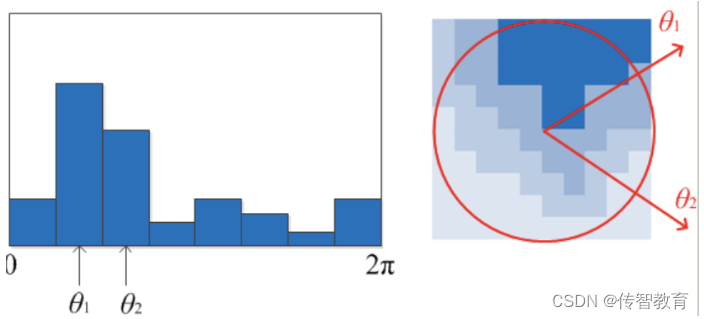
After obtaining the main direction of the key points of the image, each key point has three pieces of information (x, y, σ, θ): position, scale, and direction. From this we can determine a SIFT feature region. Usually use a circle with an arrow or directly use the arrow to indicate the three values of the SIFT area: the center indicates the feature point position, the radius indicates the key point scale, and the arrow indicates the direction. As shown below:
1.5 Description of key points
Through the above steps, each key point is assigned position, scale and direction information. Next we build a descriptor for each keypoint that is both discriminative and invariant to certain variables such as lighting, viewpoint, etc. And the descriptor not only contains the key points, but also includes the pixels around the key points that contribute to it. The main idea is to divide the image area around the key point into blocks, calculate the gradient histogram in the block, generate a feature vector, and abstract the image information.
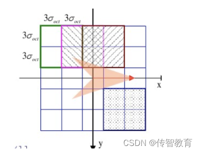
The descriptor is related to the scale of the feature point, so we generate the corresponding descriptor on the Gaussian scale image where the key point is located. With the feature point as the center, divide its neighborhood into d∗d sub-regions (generally d=4), each sub-region is a square with a side length of 3σ, considering that in actual calculation, cubic linear interpolation is required , so the feature point neighborhood is in the range of 3σ(d+1)∗3σ(d+1), as shown in the figure below:
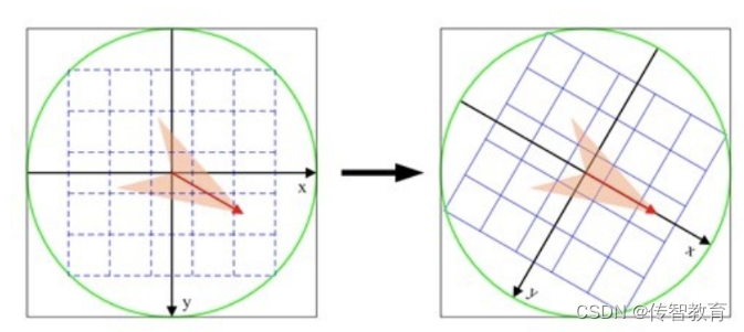
In order to ensure the rotation invariance of the feature points, take the feature point as the center, and rotate the coordinate axis to the main direction of the key point, as shown in the following figure:
Calculate the gradient of the pixels in the sub-region, and perform Gaussian weighting according to σ=0.5d, and then interpolate to obtain the gradient in eight directions of each seed point. The interpolation method is shown in the figure below:
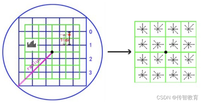
The gradient of each seed point is interpolated by the 4 subregions covering it. The red dot in the figure falls between row 0 and row 1 and contributes to both rows. The contribution factor to the seed point in row 0, column 3 is dr, and the contribution factor to row 1, column 3 is 1-dr. Similarly, the contribution factors to the two adjacent columns are dc and 1-dc, and the contribution factors to the two adjacent columns are dc and 1-dc. The contribution factors of each direction are do and 1-do. Then the final accumulated gradient size in each direction is:
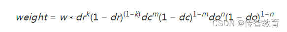
Where k, m, n are 0 or 1. The 4∗4∗8=128 gradient information counted above is the feature vector of the key point, and the feature vector of each key point is sorted according to the feature point, and the SIFT feature description vector is obtained.
1.6 Summary
SIFT has unparalleled advantages in image invariant feature extraction, but it is not perfect. There are still defects such as low real-time performance, sometimes fewer feature points, and inability to accurately extract feature points for objects with smooth edges. Since the advent of the SIFT algorithm, , people have been optimizing and improving it, the most famous of which is the SURF algorithm.