How to display the complete number in scientific notation when the number is too long in Excel

How to display the complete number in scientific notation when the number is too long in Excel

Note: The following tests are actually tested in version 16.53 of Microsoft Excel for Mac on macos, and it should be the same in windows.

1. Problem description

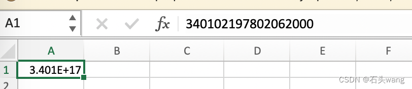
If the number is too long, it will be displayed as E+ in Excel

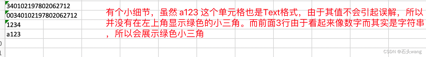
Some values, such as ID card numbers and bank card numbers, will be displayed in the form of scientific notation because the numbers are too long, where E+17 means 10 to the 17th power, as follows:

Replenish:

1. It is not only displayed in the form of E+, but more importantly, the last few digits become 0 and lose precision. The original input is 340102197802062712, and the last 3 digits become 0

2. If you enter 00340102197802062712, the leading 0 will also be ignored, and it will also become 340102197802062000 (the precision is also lost)

2. The ID number is 18 digits, and the bank card number is generally 19 digits.

In addition, the 11 digits of our mobile phone number are also easily displayed as scientific notation, but as long as the column width is increased, it can be displayed completely (but it is still regarded as a number) , as follows

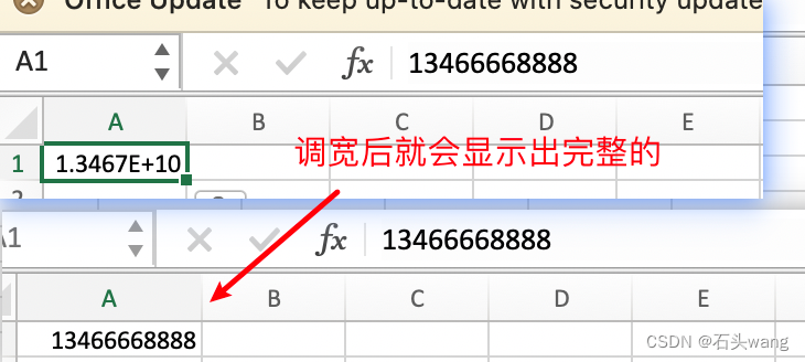
For things like ID card numbers and bank card numbers that are long to a certain length, it’s useless to adjust the width, and still display scientific notation

2. How not to display E+ (while ensuring that the 0 in front of the number is not lost, and the precision behind it is not lost)

There are several situations: 1. How to avoid copying data from other places to Excel; 2. How to change it if the number in Excel is already E+ (in this case, the 0 in front of the number has been lost, and the precision behind it has also been lost. Cooked cooked rice can only be guaranteed to be changed without E+ display)

Situation 1. Copy data from other places to Excel, and want to ensure that E+ does not appear, and the leading 0 cannot be omitted, and the precision will not be lost.

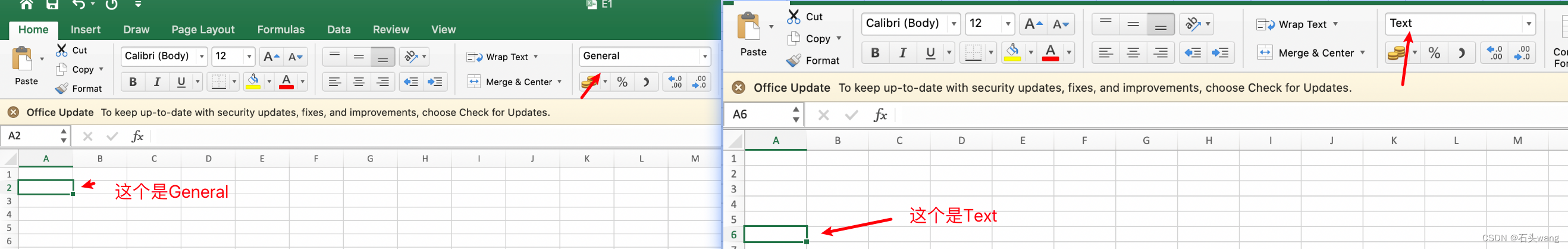
To specify the cells of Excel as Text in advance

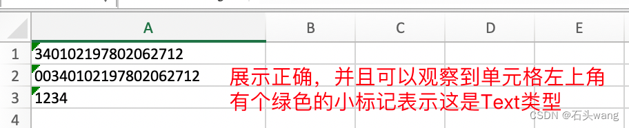
For example, if you want to copy the following values ​​into Excel

340102197802062712
00340102197802062712
1234

You have to set the format of the cell as Text in advance. For example, if you set column A as Text, and then paste it, you will get the following correct result:

If you don't set it in advance, it will look like this after pasting

Details about the small green triangle in the upper left corner of the Excel cell:

PS: How to adjust the cell format, how to know the format of the current cell?

• How to adjust cell format?

  选中要调整的单元格，可以选中整列或整行，右键 -> Format Cells... -> Number 列中选中 Text 后点击OK （我的是英文版，中文版也差不多）
  

• How to know the format of the current cell?

  

• If the selected column contains various formats, why is it shown in the above image? Answer: I don't know the rules, it's not that the display is empty, I don't know the rules

Situation 2: A certain column in Excel already contains E+ data, how to adjust it?

In this case, the 0 and precision in front of the data have been lost, and the uncooked and cooked rice cannot be rescued. The rescue here is only to display the E+ form.

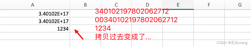
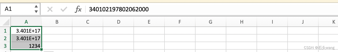
As shown in the picture,

Can "copy to plain text first, then set the text format of the cell, and then paste it back"? no! . After copying the above picture, it becomes as follows. It is useless to paste it back after setting it to Text format.

3.40102E+17
3.40102E+17
1234

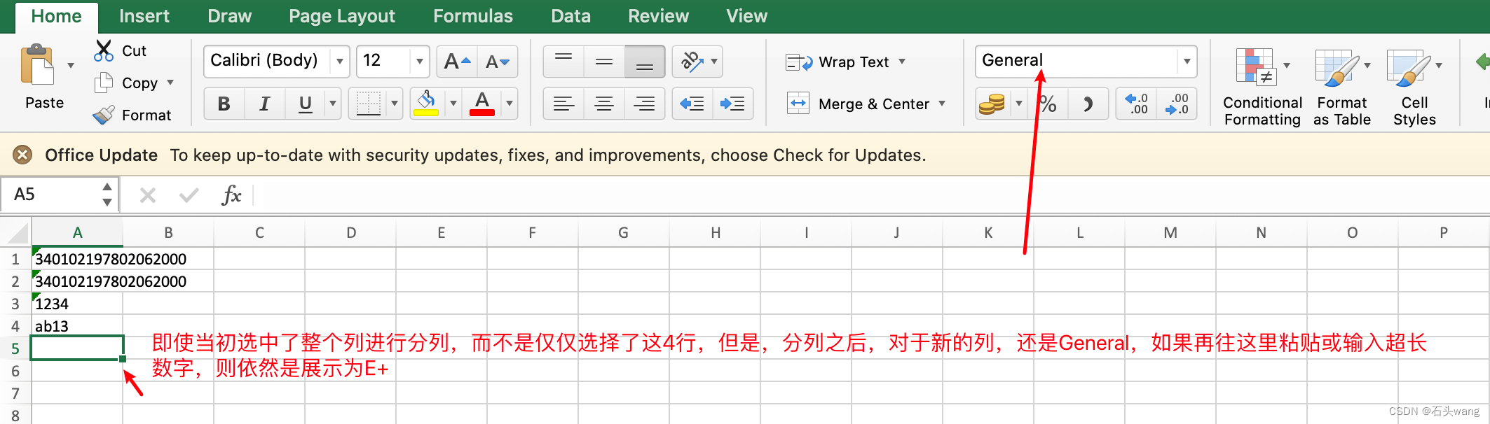
1. Method 1: Use the sorting function (most recommended)

• Select the column of E+ (you can select an entire column, or you can select the rows up to the data)
• Select the "Data" tab, select the "Text to Columns" wizard
• The first step of the wizard is to ask whether you want to use a delimiter or a fixed width to cut the data of your column, select the delimited symbol (Delimited)
• The second step of the wizard is to ask you what is the delimiter, because your data is a number, in fact, there is no delimiter, it is a whole, and you can not want to divide a column into more columns, here you can keep the default click one step
• The third step of the wizard is to ask you what format to use for the target column, of course select Text, and then click Finish

For detailed reference, there are animations here: https://www.jianshu.com/p/61790960ae62

Notice:

2. Unfeasible method: change the selected data to "text" format (this method does not work, but all the information on the Internet gives this answer)

This method cannot change the existing data, and only takes effect for new data (this statement is not entirely correct, you need to double-click the mouse line by line to display it in a non-E+ format)

3. Method 2: Use =text(A1,0) function

• Use in a new column =text(A1,0), and extend to other rows (assuming the original data is in A1)
• Copy the new column, paste it to a newer column, and choose to paste only the value when pasting, so that the formula can be eliminated

4. Method 3: Or append an empty string to become a string (=A1&"")

• Use in a new column =A1&"", and extend to other rows (assuming the original data is in A1)
• Copy the new column, paste it to a newer column, and choose to paste only the value when pasting, so that the formula can be eliminated

Other small details:

Numbers will be right-aligned by default, and strings will be left-aligned. You can use this to judge whether a string of numbers is a string or a number (but it is considered difficult to judge after adjusting the alignment method)

appendix

The better tutorials collected

https://www.jianshu.com/p/61790960ae62 (How does EXCEL convert numbers into text in batches? There are animation demonstrations )