1. Background
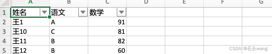
We often see that the headers of some Excel files have filtering functions, as shown in the figure.
How are these headers generated?
2. How to set the header to have filter conditions
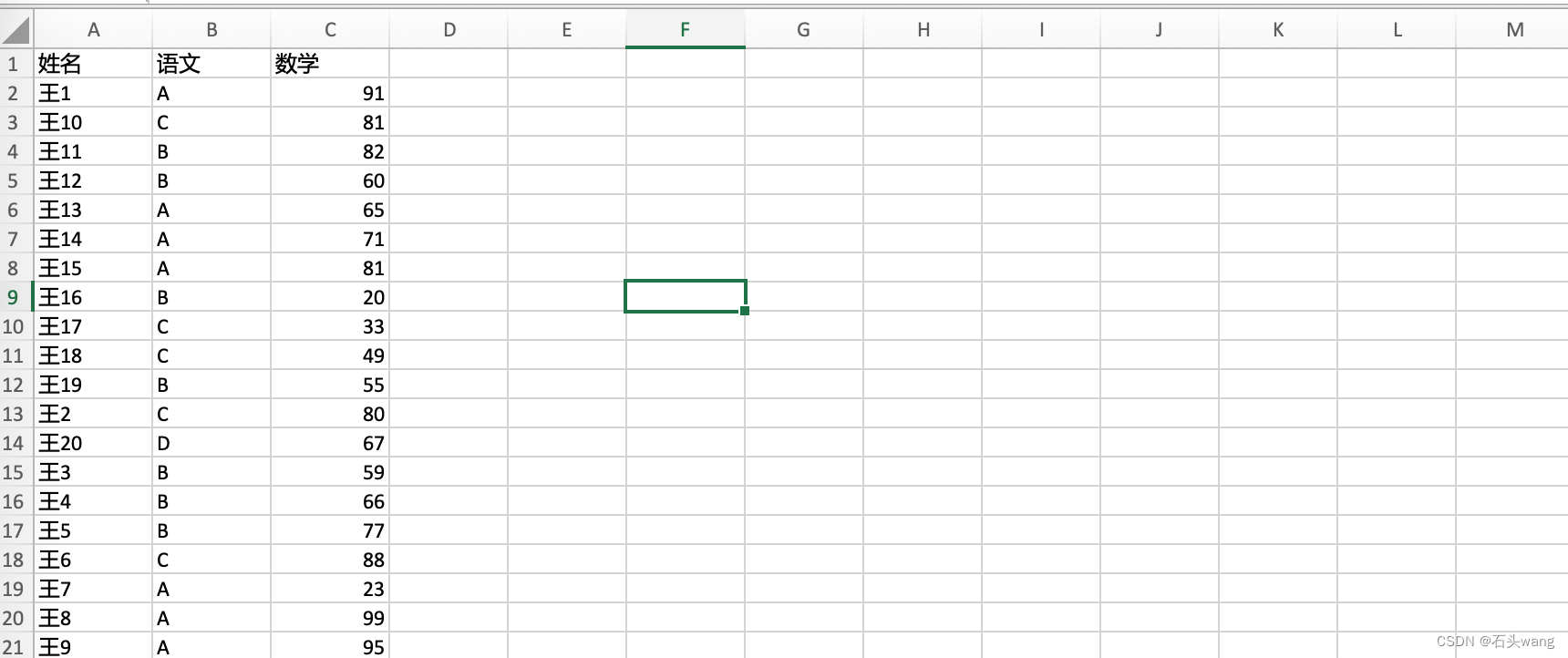
In fact, it is very simple, assuming that you already have this Excel file:
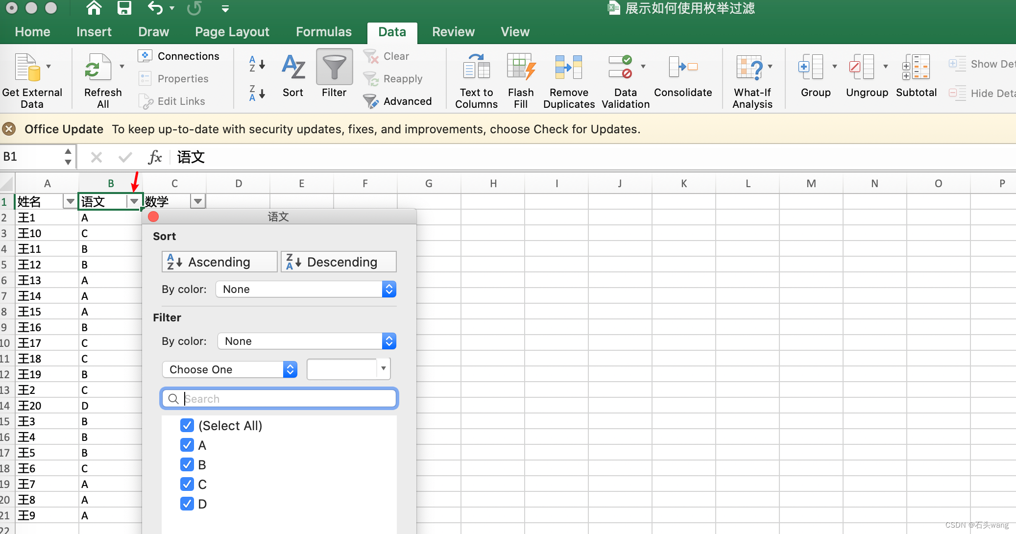
select the cell in the header (select any one) and
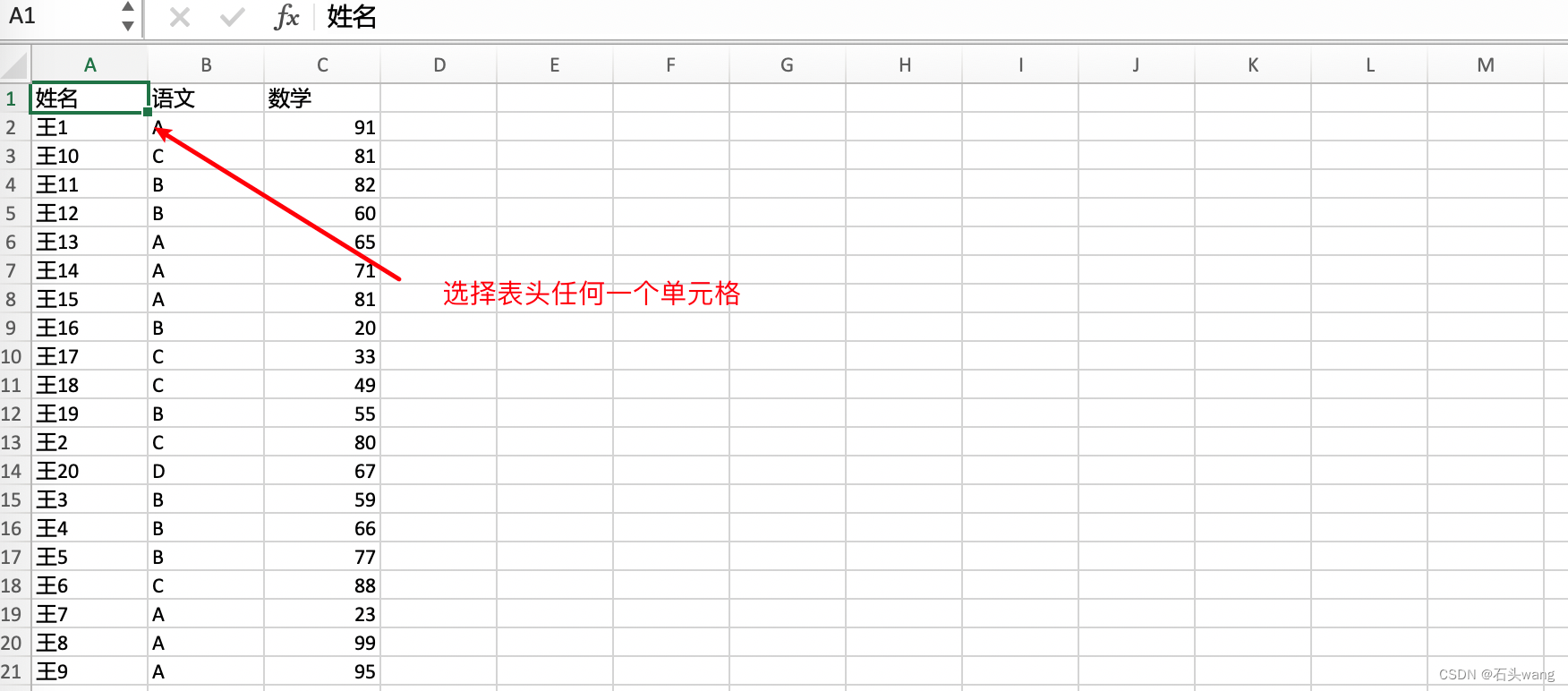
select Data->Filter (Data->Filter), then the filter conditions are generated
. You can see that each column The filter condition is actually an enumeration list composed of each value. For example, for the "language" column, there are four values (enumerations) of A, B, C, and D appearing, and you can see that there are also four filter conditions
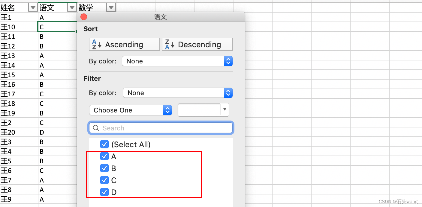
You can get what you want to check by ticking as needed.
3. About ascending and descending order and how to restore the original sort
We noticed that there is also an Ascending and Descending button that is ascending and descending. After this selection, it can be arranged in ascending or descending order.
If the ascending and descending order of the numeric type is easy to understand, if it is a string, it will be sorted in lexicographical order.
It should be noted that the original order will be disturbed after sorting, only ctrl+z can return to the original order, and the original order cannot be restored by clearing the filter conditions.
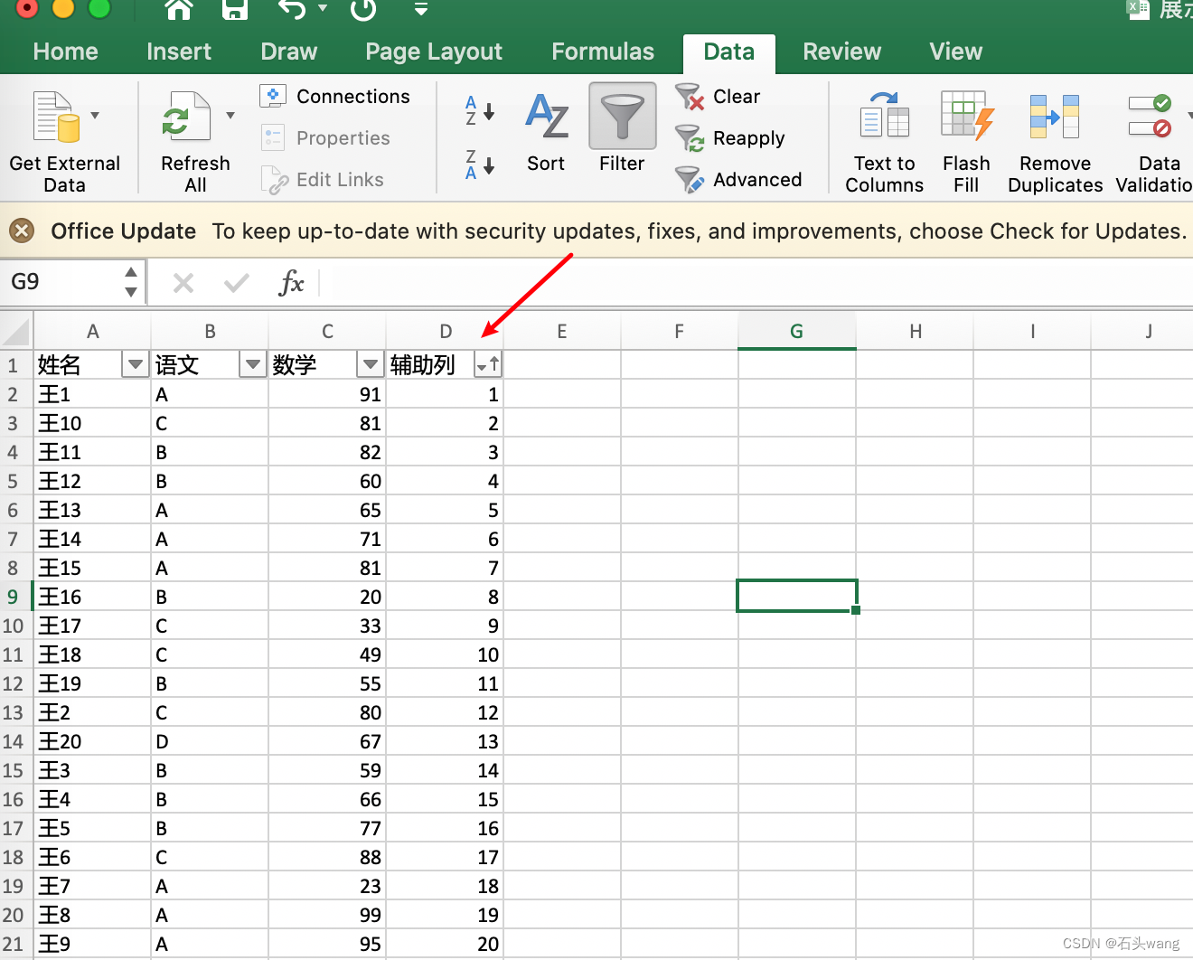
How can I restore the original order? In addition to using undo, it seems that you can only add auxiliary columns. The auxiliary columns are in the original order from 1 to n. If you want to restore the original order after sorting by "Mathematics" from high to low, you only need to follow the auxiliary columns. Sort it in ascending order
4. Supplement
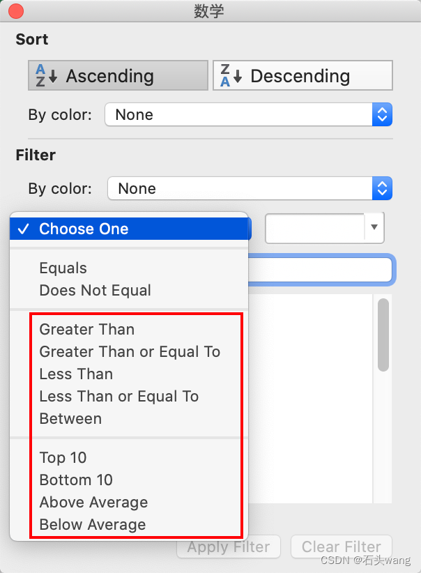
If you need to filter out students with a certain score range, you can click the filter condition
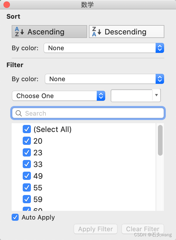
and select Choose one condition