One, the prefix and
1, prefixes and ideas
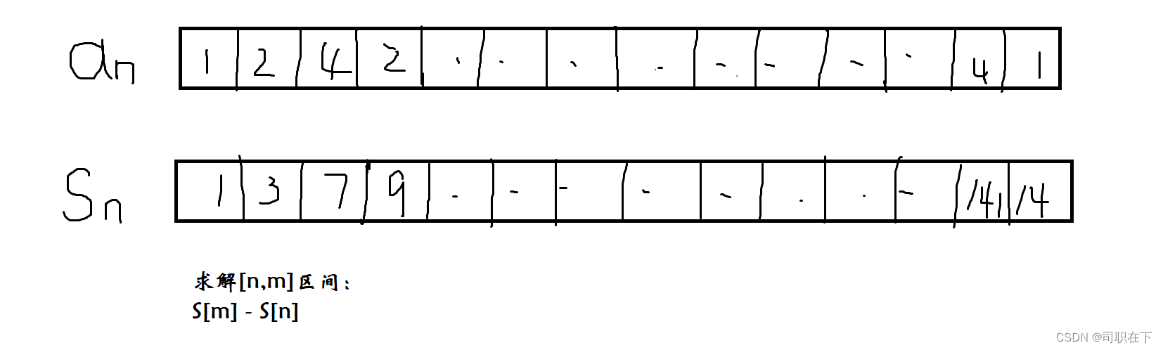
The prefix sum is a simple idea. First, we take the one-dimensional prefix sum as an example. It is used to quickly solve an interval. When we need to solve an interval, we are likely to traverse multiple times, so that the time The complexity reaches O(n) , but when this algorithm needs to be queried M times, our time complexity will accelerate, so we have a simple way to reduce this time complexity?
When we solve the interval [n, m] , we can use the idea of a m +a m-1 +...+a n in the naive algorithm to complete the naive solution to this interval. Now we want to optimize it In this process, when we read the array, we can also create an array to find the first n sums. We use this array tool and the idea of S [m] - S [n] to complete the solution of this interval.
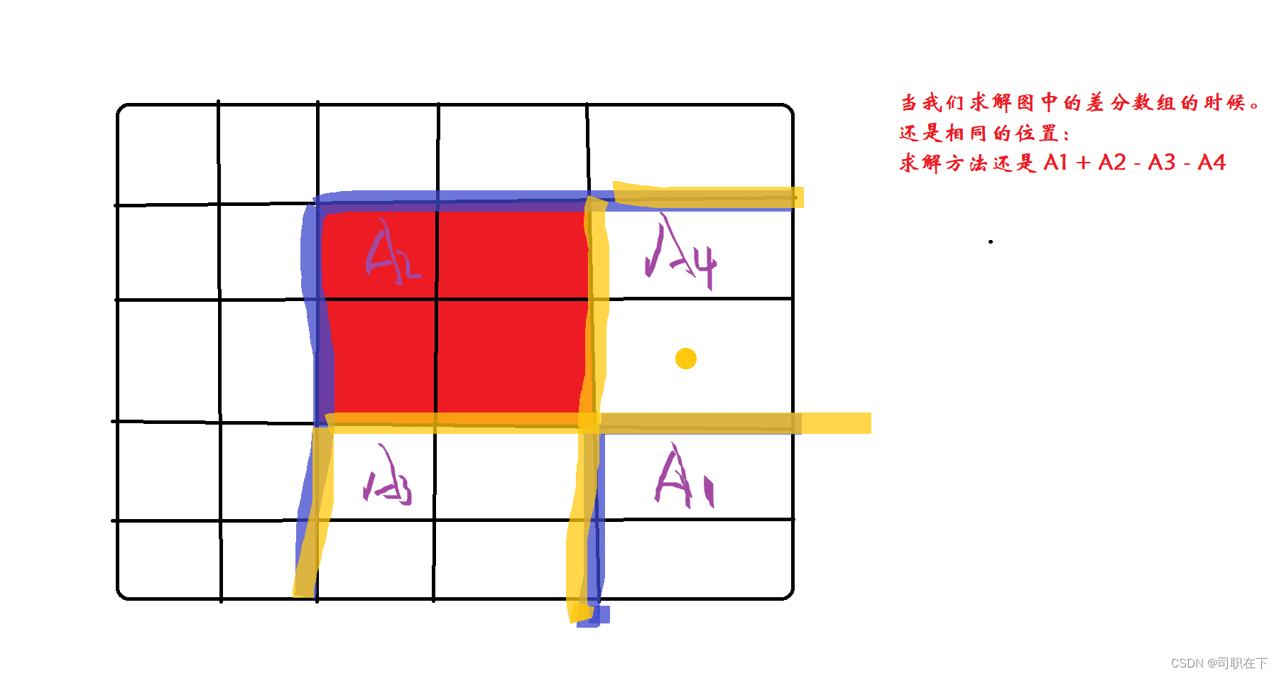
Then let's look at the two-dimensional prefix sum. The two-dimensional prefix sum is more complicated than the one-dimensional prefix sum. We can also imagine the two-dimensional array as a matrix. We can solve a prefix sum matrix for this matrix. This prefix The way to solve the sum is an idea. We can see in the following figure that we want to solve the prefix sum of the A1 area. First, we need to use the idea of A2 + A3 -A4 +D1 to solve it. D1 is the value of this point. In this way, the construction process of the two-dimensional array can be completed.
 After completing the construction process of the array, how can we solve its value in a certain area?

We can use this simulation operation to complete the processing of the two-dimensional prefix sum. When the two-dimensional prefix sum is used, we only need to follow the formula A1 + A2 -A3 -A4 to complete the logarithmic calculation operation.
2. Code implementation of prefix sum
The realization of one-dimensional prefix sum: simply write it according to the above algorithm idea, and pay attention when outputting, the operation of this output is **S[x] - S[y - 1] ** operate.
#include <iostream>
using namespace std ;
const int N = 100010 ;

int q[N] , s[N] ;
//存储该点的数值的q[N]数组,存储前缀和的s[N]数组
int main ()
{


    int n , m ;
    cin >> n >> m ;
    for(int i = 1 ; i <= n ; i ++ )
    {


        cin >> q[i] ;
        s[i] = s[i - 1] + q[i] ;
    }
    //完成两个数组的建立
    while ( m -- )
    {


        int x , y ;
        cin >> x >> y ;
        cout << s[y] - s[x - 1] << endl;
    }
    return 0 ;
}
Two-dimensional prefix sum: One thing we need to pay attention to is to prevent the occurrence of array out-of-bounds problems. Generally, we start storage operations from subscript 1 instead of subscript 0 .
#include <iostream>
using namespace std ;

const int N = 1010 ;

int q[N][N] , s[N][N] ;


int main ()
{

    ios::sync_with_stdio(0);
    int n , m , cnt ;
    cin >> n >> m >> cnt ;
    for(int i = 1 ; i <= n ; i ++ )
        for(int j = 1 ;j <=m ;j ++ )
            cin >> q[i][j] ;
//完成q数组的构建
        for(int i = 1 ; i <= n ; i ++ )
        for(int j = 1 ;j <=m ;j ++ )
            s[i][j] = s[i - 1][j] + s[i][j -1] + q[i][j] - s[i - 1][j - 1] ;
//完成s数组的构建
        while (cnt -- )
            {


                int x1, x2, y1 , y2 ;
                cin >> x1 >> y1 >> x2 >> y2 ;
                cout << s[x1 - 1][y1 - 1] + s[x2][y2] - s[x1 - 1][y2] - s[x2][y1 - 1] << endl ;
            }

    return 0 ;
}
Second, the difference algorithm
1, Difference algorithm idea
The difference algorithm is to solve the interval operation, and the prefix sum is to solve the interval summation. The so-called difference is to open a related array to store the difference between this digit and the previous digit, so as to perform related operations. The first is the one-dimensional prefix sum. We only use q[n] - q[n -1] to complete the storage operation of the array. When we perform interval operations and add x to the [n,m] interval , we The idea is that c[n] += x , c[m + 1] -= x . When we output this array, we can output it by adding step by step,
The two-dimensional difference array is relatively complicated. The two-dimensional difference cannot be thought of like the two-dimensional prefix sum. These two can be said to be two things with different ideas. The two-dimensional difference array is a backward operation. First, the two phases The added arrays are a[x1][y1] and **a[x2 + 1][y2 + 1]**, the operation of subtraction is the operation of adding a very large one, we can see that the following array is basically
a It perfectly interprets the difference operation, which explains the read-in operation of the difference matrix, but it has not completed its output operation, and its output operation should be an operation similar to the prefix sum on both sides and subtraction on the diagonal.
2. Realization of difference algorithm
One-dimensional difference algorithm
#include <iostream>
using namespace std ;

const int N  =100010 ;

int q[N] , k[N] ;

int main ()
{


    int n , m ;
    cin >> n >> m;
    for(int i = 1 ; i <= n ;i ++ )
    {


        cin >> q[i] ;
        k[i] = q[i] - q[i - 1] ;
    }

    //完成原数组和差分数组的赋值操作
    while ( m -- )
    {


        int x ,y , z ;
        cin >> x  >> y >> z;
        //核心步骤
        k[x] +=z ;
        k[y + 1] -= z ;
        //以上两步
    }
    int cnt = 0 ;
    for(int i = 1 ; i <= n ; i ++ )
        {


            cnt +=k[i];
            cout << cnt << " ";
        }
    return 0 ;
}
2D Difference Algorithm
#include <iostream>

using namespace std ;

const int N = 1010 ;

int q[N][N] , k[N][N] ;

void insert (int x1 ,int y1 ,int x2 ,int y2 ,int z)
{


    k[x1][y1] += z;
    k[x2 + 1][y2 + 1] += z ;
    k[x2 + 1][y1] -= z ;
    k[x1][y2 + 1] -= z ;
}

int main ()
{


    int n , m , p ;
    cin >> n >> m >> p;
    for(int i = 1 ; i <= n ; i ++ )
        for(int j = 1 ; j <= m ; j ++ )
            {

    cin >> q[i][j] ;
            insert(i , j , i , j,q[i][j]);
            }
        while (p --)
        {


            int x1 ,y1, x2 ,y2 ,cnt ;
            cin >> x1 >> y1 >> x2 >> y2 >> cnt ;
            insert(x1 ,y1 ,x2 ,y2 ,cnt );
        }
        for(int i = 1 ;i <= n ;i ++ )
           {

     for(int j = 1 ;j <= m ;j ++ )
            {


                k[i][j] +=  k[i - 1][j] + k[i][j - 1]- k[i -1 ][j - 1];
                cout << k[i][j] << " ";
            }
            cout << endl;
        }
    return 0 ;
}
Three, the thinking of two algorithms
Whether it is the differential algorithm or the prefix sum algorithm, they all focus on completing the operation of this algorithm through an array tool. We only need to master the creation of these arrays, the use of intervals, and the output operation to complete the understanding of these algorithms. At the same time, the prefix The sum and difference array are opposite, so the creation of the prefix sum is actually equivalent to the output of the difference (advanced version, to assign a value to the difference array) and the creation of the difference is also similar to the output of the prefix sum (not exactly the same)