Summary: Skin color and roughness are visually distinct. When image processing involves skin analysis, it is important to quantitatively assess this difference using texture features. In this paper, we discuss a statistical approach to texture analysis and measurement pattern recognition. Grain size and anisotropy were assessed with appropriate diagrams. The possibility of determining the presence of pattern defects is also discussed.
Key words: two-dimensional texture; skin texture; texture function; defect localization
1 Introduction
Quantitative characterization of human skin texture is one of the tasks involved in image processing recently. There are two interesting things about this problem of texture analysis. In addition to computational modeling of realistically rendered skin in computer graphics [1], we must also consider the possibility of applying texture analysis to computer-aided diagnosis in dermatology [2, 3].
Skin texture is the smooth appearance of the skin's surface. For the characteristics of this texture, many factors go into play, such as diet and hydration, the amount of collagen and hormones, and of course skin care. In addition, the skin gradually decays with age. As skin ages, it becomes thinner, more easily damaged, and wrinkled. This deterioration is also accompanied by a darkening of skin color as the skin's topmost cell layer overabsorbs the natural pigment melanin. Skin texture also depends on its body location. In the case of image processing, we have to take into account the fact that the appearance of textures varies with image recording parameters, i.e. camera, lighting and viewing angle, a problem common to any real surface.
The task of quantitative assessment of skin features is rather complex, since in all cases image analysis has to be applied to surfaces with irregular, aperiodic patterns.
For skin texture, methods based on wavelets [8], adaptive segmentation [9] and genetic image analysis [10] have been proposed. References [11] and [12] characterized skin topography by processing skin contours obtained with capacitive devices to study skin aging. Here we propose to apply Skin Representation, an image processing procedure previously used to study texture transitions in nematic liquid crystals [13–14]. This treatment is suitable for images with smooth, almost irregular textures, such as those observed in microscopic studies of certain nematic liquid crystal cells. This processing is based on coherence length analysis, described in detail in the next section.
2. Image Analysis
For each pixel at any point P(x, y) in the image frame, we associate it with a gray level b in the range 0 to 255: b(x, y) is a binary number representing the intensity (brightness) distribution of the image dimension function. Starting from the function b(x,y) given the gray level of a pixel, the following calculations can be performed. First, determine the average intensity of the pixel hue:

where lx, ly are the x and y rectangular extents of the image frame. More generally, the k-th order statistical moments of an image are defined in the following way:

With this characterization, we are able to define the mean value of the moments of the entire image frame. A distribution of pixel hues is then given from these moments. It turns out that the tonal dispersion is evaluated by k=2 moments.
All integrals can be computed over the entire image or over a window. In the case of windowing the image, the moments Mo and Mk allow to find the position and shape of the object, since the distribution can be changed for each specific window. In images where no particular object is present at first glance, we can use the same values of the moments Mo and Mk defined by equations (1) and (2) for the entire image, assuming the image is characterized by a single intensity distribution. However, to determine whether an image exhibits irregular domains or localized defects, it is useful to estimate the mass ratio between the intensity standard deviation and the average intensity value over the entire image frame within a fixed acceptable limit, such as 50%.
Let us emphasize the fact that a domain can be described by an intensity distribution that can be substantially different from those of other domains or the background distribution. In this case, it is misleading to proceed from the point of view that only one distribution is sufficient to describe the entire image frame. Instead, in this case it is necessary to share the image in a grid of windows, where within each window the mass ratio is below the acceptable limit. The choice of limit values does not affect the sensitivity of the method, since the choice related to the range of statistical variables for subdivided categories also does not affect the location of the sample and the dispersion index.
However, it is necessary to check that the homogeneity assumption is actually validated and that the preferred orientation is shown in the image box (assumption of isotropy). We introduced a typical length characterizing the texture size, which is very useful for the characterization of smectic and nematic phases [13, 14].
Instead of measuring homogeneity, we compute the intensity difference entropy of the histogram versus the distance to a point in the image frame (see e.g. [15]), or by computing the spatial organization through "travel statistics" [16, 17]. A set of coherence lengths defined in the following way. Starting from an arbitrary point P(x,y) of graph b(x,y), along several radial directions, we calculate the values of Moi(x,y) and Mki(x,y) moments, namely:

Among them, the index i is in the radial direction, r is the radial distance from P, and θi is the angle formed by the i direction and the y-axis (see Figure 1 for the reference system). The lengths lo,i and lk,i are the radial distances (from P) at which the values of the moments Moi(x,y) and Mki(x,y) in the chosen direction are at the threshold level t Inner saturation to image average moments Mo and Mk. This is how you define the local "coherence lengths" lo,i(x,y) and lk,i(x,y) of a point P in an image frame. The choice of threshold t depends on the problem under study.
In the calculation of the functions lo,i(x,y) and lk,i(x,y), pixels near the boundaries of the image frame are not involved, since in this case it is not possible to estimate the coherence length in all directions (boundary effect). In contrast, in standard image processing techniques [18], the periodicity of the image, either initially present or artificially introduced by duplicating frames, is used to overcome the boundary problem. Let us emphasize the fact that the moments Moi(x,y) and Mki(x,y) are not calculated over windows in the image frame, but in specific directions: thus, the method differs from standard statistical methods , allowing to account for anisotropy in texture recognition problems in a natural way. In our analysis, we will use the 32 directions in Figure 1.

Figure 1: The reference system used to calculate the mean value along the i direction. In the figure we show the 32 directions used in the evaluation of the coherence length map.
In fact, we can look for anomalous behavior of the vector lo,i(x,y) or lk,i(x,y) as a signal of a defect in the position of the image frame corresponding to a given point P(x,y), for For each specific i direction:

[Note 1: The coherence length is a well-known concept in optics and condensed matter physics. In optics, it is the propagation distance from a coherent source to the point at which electromagnetic waves maintain a certain degree of coherence. In condensed matter physics, it's the distance that maintains order. For example, we can tell that we are coherent in a state of matter when we have a long-range atomic or molecular order. The coherence length is significantly larger than the molecular size. In general, coherence length refers to the size of the ordered domains in materials where long-range order occurs, such as ordered domains in liquid crystals. The term coherence length is also used to characterize the scale of the distribution of average molecular orientation in a distorted transition layer formed at a solid/liquid crystal interface when an electric or magnetic field is applied. ]
If the image frame is strictly uniform, such an average length should coincide with the actual local length measured for all image points. On the other hand, if the image frames are completely non-uniform, the local lengths will be very scattered around their mean value. The same happens when image frames are shared in windows, each with a different intensity distribution. If the image can be considered to be characterized by only one distribution over a reasonable range of dispersion, the coherence length can be averaged over the entire image frame. The length Lo,i represents the distance along the direction i from the general point P(x,y) to where the image intensity actually reaches the mean value: this means that the distance depends on the threshold level.

Figure 2: Coherent length diagrams for two snakeskins from the Brodatz album (right). The inner curve corresponds to a threshold of 0.5 and the outer curve to 0.2
. Numbers on the axes correspond to pixel numbers. Note that this plot is able to indicate texture anisotropy. For a chosen threshold, the graph is the boundary of the smallest region with the same feature characterizing the entire image frame.
In Fig. 2, the average Lo,i of two snakeskin images from the Brodatz album is reported. The result is a schematic diagram of Lo,i in the 32 directions in Fig. 1. We can define this graph as a "coherence length graph". In fact, the figure shows two plots obtained by fixing two different thresholds. To obtain the inner map, we use a threshold corresponding to 50% of the ratio. External charts were obtained with 20% of the same scale. These maps reveal the preferential directions in the image texture, i.e. the anisotropy of the texture.
In this paper, we only consider Lo,i since this gives the most intuitive results. A graph of length Lo,i represents the smallest region about a general point P(x,y) over which we obtain a value Mo within a fixed threshold level when evaluating the average value of pixel intensities. The graph represents the boundaries of image unit regions that contain typical features of the entire image, and we can easily compare the graph to snake scales. In fact, the unit area appears as a primitive unit cell in a lattice (see ref. 19 for a description of a unit cell in a lattice). We can also view this area or coherence length map as a measure of grain size and then evaluate the roughness of the image texture.
A defect in the image texture can be thought of as any object in the image frame that has a different shape, e.g. a different shape from the cell, or a different cell average hue, etc.
3. Skin texture analysis and discussion
The case of snakeskin gives a diagram that immediately recalls the properties of the unit cells in the lattice. This is because textures are quite geometric. Of course, the characteristics of human skin are different, but as we have observed from its use in liquid crystal microscopy studies [13, 14], it is in the case of almost homogeneous images that Fourier analysis is almost inactive and coherent Length is useful.
We analyzed images of humanoid textures with coherence length (Lo,i) plots, and the results are shown in Figure 3, in the middle of the plot. In the lower part of the figure, the leather texture and corresponding analysis are shown. The inner and outer curves have thresholds, which are used to obtain the graph of Figure 2. The shape of the two graphs has not changed substantially. The area is changing: this is because a larger area is required to achieve a lower threshold.
On the right side of the figure, we see the detection of defects: points marked in red are considered "defects", while pixels marked in green are normal. This is not a segmentation process at the origin of the red-green map, but a criterion of local behavior involving the coherence length lo,i(x,y). In the case we are discussing, i.e. the case of almost homogeneous image frames, we reasonably assume that the point P(x,y) does not belong to the defect, if the average local value is defined as:

Included between the two extreme lengths Lo,min and Lo,max, where Lo,min is the minimum of the 32 averages of equation (5) and Lo,max is the maximum. Obviously, for almost isotropic image frames, the two extreme values Lo,min and Lo,max are close together.
At points marked in red (i.e. defects), the average local coherence length lo(x,y) is not included in the interval [lo,min,lo,max]. Conversely, points that are not defects are marked in green. We use red and green halftones to see the original texture in this defect image.
For commercial software, a common procedure for identifying defects is based on grayscale thresholding [15]: this means a procedure that checks whether the intensity of a pixel is consistent with a specific chosen grayscale within a fixed tolerance. This process is called "image segmentation by thresholding" and generates an image segmented in two or more regions according to the thresholding used. This technique doesn't investigate the neighborhood of a pixel, so there's no way to determine if it's actually a defect. Through the analysis discussed in this paper, defect detection is to compare the local coherence length lo,i(x,y) of the local unit with the coherence length lo,i map and the global unit, as shown in the middle of Fig. 3. We then compare the behavior of the pixel neighborhood to the average behavior of all pixel neighborhoods.

Figure 3: In the middle of the figure, we can see the coherence length maps of two humanoid skin textures and one leather texture (below). The inner and outer curves have thresholds, as shown in Figure 2. On the right side of the figure, we see the detection of "defects". Points marked in red are considered "defects" (see text for explanation). Let us note that this is not a segmentation thresholding procedure as it is available through commercial programs.
For example, in the case of human skin, defects could be areas of lighter or darker color, or areas with wrinkles. In the upper part of Figure 3 we see an almost regular texture with a darker area. The coherence length plot shows that the texture is isotropic and we actually have no wrinkles. Defect maps obtained as described previously demonstrate darker regions.
Figure 3 shows a slightly anisotropic unit cell with a wrinkled texture, as shown in the coherence length plot (see middle of figure). Ignoring this anisotropy, the process of defect detection can see regions with different intensities in the background. A procedure could be developed to compare the true shape of the local and global coherent regions, but this is the subject of further research. There are no wrinkles on the leather surface, which then appear as the upper picture in the same picture. We can consider this defect detection procedure as a good method for fault detection in the leather industry.
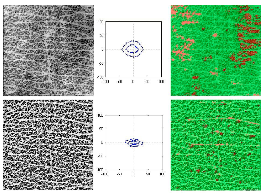
Figure 4: Coherence length map evaluation can be used on maps obtained by capacitive systems (ref. 11). The thresholds for these maps are shown in Figures 2 and 3. The upper left image shows a map of the capacitive system. In the lower part of the figure, we see the same image after image contrast normalization. Note that the graphs are different due to the different distribution of pixel tones. This difference is enhanced by the defect detection procedure (the procedure is the same as in Fig. 3). In the upper part, we see the concentration of red areas where the renormalization routine must work in changing the distribution of pixel tones. In lower images, the number of defects is greatly reduced.
Coherence length maps of maps obtained from capacitive systems can also be obtained (see ref. 11). In the upper part of Figure 4 we can see the mapping of the capacitive system. In the bottom half we see the same image after image contrast normalization: the capacitive image is sensitive to differential hydration and the presence of sweat, which produces darker areas that then need to be renormalized.
Note that the coherence length plots are different because the pixel tone distribution is different. This difference is demonstrated by our previous defect detection procedure for the texture shown in Figure 3. In the upper right part of Figure 4, we see red areas concentrated where the normalization process must more forcefully alter the distribution of pixel tones to obtain a renormalized image. Therefore, the bottom right image, the defect map of the re-malignant image, shows a small number of defects.
The aim of Ref. 11 was to develop a device for characterizing skin topography to measure skin contour and the presence of wrinkles. Image renormalization is necessary for the segmentation of skin topography to correlate it with skin aging. In the case of dealing with images recorded by a camera, where illumination and perspective are important, a similar normalization procedure is useful.
Our image analysis of skin texture is based on the evaluation of the global gray level distribution across the image frame, and then on a coherence length map capable of revealing texture anisotropy. These charts also enable the estimation of texture characteristics such as anisotropy and roughness: these charts can then adequately describe the presence of wrinkles. Depending on the chosen statistical parameters of the gray distribution, several defect detection methods can be proposed. We followed a simple procedure that was able to identify local differences from the background, but more complex procedures could easily be adapted based on clinical experience.