Introduction to Deep Learning (60) Recurrent Neural Network - Gated Recurrent Unit GRU

foreword

The core content comes from blog link 1 blog link 2 I hope you can support the author a lot
This article is used for records to prevent forgetting

Recurrent Neural Network - Gated Recurrent Unit GRU

courseware

focus on a sequence

Not every observation is equally important.

Wanting to remember only relevant observations requires:

• Mechanisms that can be followed (update gate)
• Forgetting Mechanism (Reset Gate)

Door

candidate hidden state

hidden state

Summarize

$$\begin{array}{r}\begin{array}{r}{\mathbf{R}}_t=s(X_t{\mathbf{W}}_{xr}+{\mathbf{H}}_{t-1}{W}_{hr}+{\mathbf{b}}_r),\\ {\mathbf{Z}}_t=s(X_t{\mathbf{W}}_{xz}+{\mathbf{H}}_{t-1}{W}_{hz}+b_z),\\ \mathrm{fishy}({X\; .)}_t{W}_{xh}+\left({\mathbf{R}}_t\odot H_{t-1}\right)W_{hh}+b_h),\\ H_t=Z_t\odot H_{t-1}+(1-Z_t)\odot {\tilde{H}}_t.\end{array}\end{array}$$

Textbook

In the section Backpropagation through Time, we discussed how gradients are computed in recurrent neural networks, and the problem that successive matrix products can lead to vanishing or exploding gradients. Let's briefly think about the significance of this gradient anomaly in practice:

• We may come across situations where early observations are very important for predicting all future observations. Consider an extreme case where the first observation contains a checksum and the goal is to discern at the end of the sequence whether the checksum is correct. In this case, the influence of the first lemma is crucial. We would like to have some mechanism for storing important early information in a memory cell. Without such a mechanism, we would have to assign a very large gradient to this observation, since it would affect all subsequent observations.

• We may encounter situations where some tokens have no associated observations. For example, when sentiment analysis is performed on webpage content, there may be some auxiliary HTML codes that have nothing to do with the sentiment conveyed by the webpage. We would like to have some mechanism to skip such tokens in the hidden state representation.

• We may encounter situations where there are logical breaks between parts of the sequence. For example, there may be transitions between chapters of a book, or between bear and bull markets in a security. In this case, it would be nice to have a way to reset our internal representation of state.

Many methods have been proposed in academia to solve such problems. One of the earliest methods is "long-short-term memory" (long-short-term memory, LSTM). A gated recurrent unit (GRU) is a slightly simplified variant that generally provides equivalent performance and is significantly faster to compute. Since the gated recurrent unit is simpler, we start with it.

1 Gated hidden state

The key difference between Gated Recurrent Units and ordinary RNNs is: The former supports gating of hidden states. This means that the model has specialized mechanisms for determining when the hidden state should be updated, and when the hidden state should be reset. These mechanisms are learnable and address the problems listed above. For example, if the first token is very important, the model will learn not to update the hidden state after the first observation. Likewise, the model can also learn to skip irrelevant casual observations. Finally, the model will also learn to reset the hidden state when needed. Below we discuss the various types of gating in detail.

1.1 Reset Gate and Update Gate

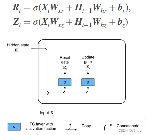
We first introduce 重置门（reset gate）and update the gate （update gate）. We design them as $(0,1)$ vectors in the interval so that we can do convex combinations. The reset gate allows us to control how much of the past state we "might still want to remember"; the update gate will allow us to control how many of the new state are copies of the old state.

We start by constructing these gates. The figure below describes the input of the reset gate and update gate in the gated recurrent unit. The input is given by the input of the current time step and the hidden state of the previous time step. The outputs of the two gates are given by two fully connected layers using the sigmoid activation function.

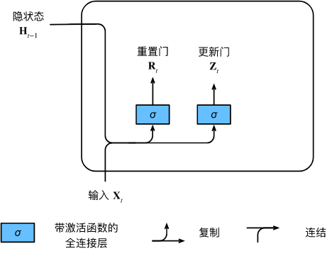
Let's look at the mathematical representation of a gated recurrent unit. For a given time step $t$ , assuming the input is a mini-batch${\mathbf{X}}_t\in {\mathbb{R}}^{n\times d}$ (number of samples$n$ , input number$d$ ), the hidden state of the last time step is${\mathbf{H}}_{t-1}\in R^{n\times h}$ (number of hidden units). Then, the reset gate$R_t\in R^{n\times h}$ and update gate${\mathbf{Z}}_t\in R^{}$Determine the function of${}^n$${}^{\times }$${}^h$
$$\begin{array}{r}\begin{array}{r}{\mathbf{R}}_t=s(X_t{\mathbf{W}}_{xr}+{\mathbf{H}}_{t-1}{W}_{hr}+{\mathbf{b}}_r),\\ {\mathbf{Z}}_t=s(X_t{W}_{xz}+H_{t-1}{W}_{hz}+b_z),\end{array}\end{array}$$
For ${\mathbf{W}}_{xr},W_{xz}\in {\mathbb{R}}^{d\times h}$和$W_{hr},W_{hz}\in R^{h\times h}$ is the weight parameter,${\mathbf{b}}_r,b_z\in R^{1\times h}$ is the bias parameter. Note that a broadcast mechanism is triggered during the summation. We use the sigmoid function to convert the input value to the interval$(0,1)$。

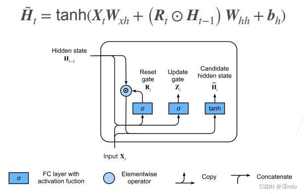
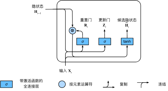
1.2 Candidate Hidden States

Next, let's reset the gate $R_t$与RNN中${\mathbf{H}}_t=\varphi (X_t{\mathbf{W}}_{xh}+H_{t-1}{W}_{hh}+{\mathbf{b}}_h).$ Integrating the regular hidden state update mechanism in ., get at time step$t$的候选隐状态（candidate hidden state） ${\tilde{H}}_t\in {\mathbb{R}}^{n\times h}$
$${\tilde{H}}_t=\mathrm{fishy}({X\; .)}_t{W}_{xh}+\left({\mathbf{R}}_t\odot {\mathbf{H}}_{t-1}\right){\mathbf{W}}_{hh}+{\mathbf{b}}_h),$$
其中$W_{xh}\in {\mathbb{R}}^{d\times h}$和$W_{hh}\in R^{h\times h}$ is the weight parameter,$b_h\in R^{1\times h}$ is a bias item, symbol$\odot$ is the Hadamard product (element-wise product) operator. Here, we use the tanh non-linear activation function to ensure that the values ​​in the candidate hidden states remain in the interval$(-1,1)$ .

与${\mathbf{H}}_t=\varphi (X_t{\mathbf{W}}_{xh}+H_{t-1}{W}_{hh}+{\mathbf{b}}_h).$ Compared with the R t \mathbf{R}_tin the above formula${\mathbf{R}}_t$和$H_{t-1}$Multiplying the elements of can reduce the influence of previous states. Whenever the reset gate $R_t$When the term in is close to 1, we restore a normal recurrent neural network as in a normal RNN. For the reset gate $R_t$All close items in 0, the candidate hidden state is ${\mathbf{X}}_t$The result of the multilayer perceptron as input. Therefore, any pre-existing hidden state is ** 重置** ** the default value.

The figure below illustrates the computation flow after applying the reset gate.

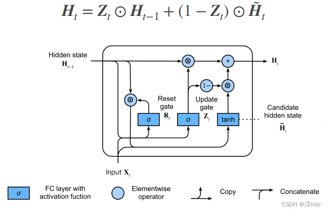
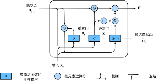
1.4 Hidden state

The above calculation results are only candidate hidden states, we still need to combine the update gate ${\mathbf{Z}}_t$Effect. This step determines the new hidden state ${\mathbf{H}}_t\in {\mathbb{R}}^{To\; what\; extent\; n\times h}$ comes from the old state$H_{t-1}$and a new candidate state ${\tilde{H}}_t$. Update gate ${\mathbf{Z}}_t$Only need in $H_{t-1}$和${\tilde{H}}_t$This goal can be achieved by performing an element-wise convex combination between them. This leads to the final update formula for the gated recurrent unit: $$H_t=Z_t\odot H_{t-1}+(1-Z_t)\odot {\tilde{H}}_t.$$
Whenever update gate$Z_t$When it is close to 1, the model tends to keep only the old state. At this point, from ${\mathbf{X}}_t$The information of is essentially ignored, effectively skipping time step t in the dependency chain. On the contrary, when ${\mathbf{Z}}_t$When close to 0, the new hidden state ${\mathbf{H}}_t$It will be close to the candidate hidden state ${\tilde{H}}_t$. These designs can help us deal with the vanishing gradient problem in recurrent neural networks and better capture the dependencies of sequences with long time step distances. For example, if the update gate is close to 1 for all time steps of the entire subsequence, the old hidden state at the beginning time step of the sequence will be easily retained and passed to the end of the sequence, regardless of the length of the sequence.

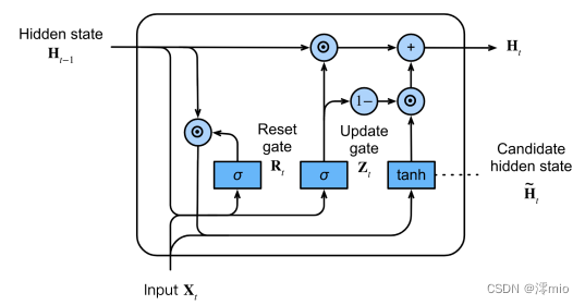
The figure below illustrates the computation flow after the update gate is in effect.

In summary, gated recurrent units have the following two salient features:

• Reset gates help capture short-term dependencies in sequences;

• Update gates help capture long-term dependencies in sequences.

2 Implementation from scratch

To better understand the gated recurrent unit model, we implement it from scratch. First, we read the Medium Time Machine dataset:

import torch
from torch import nn
from d2l import torch as d2l

batch_size, num_steps = 32, 35
train_iter, vocab = d2l.load_data_time_machine(batch_size, num_steps)

2.1 Initialize model parameters

The next step is to initialize the model parameters. We draw weights from a Gaussian distribution with a standard deviation of 0.01 and set the bias term to 0, hyperparameters num_hiddensdefine the number of hidden units, instantiate all weights related to update gate, reset gate, candidate hidden state and output layer and bias.

def get_params(vocab_size, num_hiddens, device):
    num_inputs = num_outputs = vocab_size

    def normal(shape):
        return torch.randn(size=shape, device=device)*0.01

    def three():
        return (normal((num_inputs, num_hiddens)),
                normal((num_hiddens, num_hiddens)),
                torch.zeros(num_hiddens, device=device))

    W_xz, W_hz, b_z = three()  # 更新门参数
    W_xr, W_hr, b_r = three()  # 重置门参数
    W_xh, W_hh, b_h = three()  # 候选隐状态参数
    # 输出层参数
    W_hq = normal((num_hiddens, num_outputs))
    b_q = torch.zeros(num_outputs, device=device)
    # 附加梯度
    params = [W_xz, W_hz, b_z, W_xr, W_hr, b_r, W_xh, W_hh, b_h, W_hq, b_q]
    for param in params:
        param.requires_grad_(True)
    return params

2.2 Define the model

Now we will define the initialization function for the hidden state init_gru_state. Like the function defined in section RNN Implementation from Zero init_rnn_state, this function returns a （批量大小，隐藏单元个数）tensor of shape , whose values ​​are all zeros.

def init_gru_state(batch_size, num_hiddens, device):
    return (torch.zeros((batch_size, num_hiddens), device=device), )

Now we are ready to define the Gated Recurrent Unit model. The architecture of the model is the same as the basic RNN unit, except that the weight update formula is more complicated.

def gru(inputs, state, params):
    W_xz, W_hz, b_z, W_xr, W_hr, b_r, W_xh, W_hh, b_h, W_hq, b_q = params
    H, = state
    outputs = []
    for X in inputs:
        Z = torch.sigmoid((X @ W_xz) + (H @ W_hz) + b_z)
        R = torch.sigmoid((X @ W_xr) + (H @ W_hr) + b_r)
        H_tilda = torch.tanh((X @ W_xh) + ((R * H) @ W_hh) + b_h)
        H = Z * H + (1 - Z) * H_tilda
        Y = H @ W_hq + b_q
        outputs.append(Y)
    return torch.cat(outputs, dim=0), (H,)

2.3 Training and Prediction

Training and prediction work exactly the same as before. After training, we print out the perplexity on the training set and the perplexity on the predicted sequences prefixed with "time traveler" and "traveler", respectively.

vocab_size, num_hiddens, device = len(vocab), 256, d2l.try_gpu()
num_epochs, lr = 500, 1
model = d2l.RNNModelScratch(len(vocab), num_hiddens, device, get_params,
                            init_gru_state, gru)
d2l.train_ch8(model, train_iter, vocab, lr, num_epochs, device)

output:

perplexity 1.3, 28030.1 tokens/sec on cuda:0
time traveller wetheving of my investian of the fromaticalllesp
travellery celaner betareabreart of the three dimensions an

3 Concise implementation

The high-level API contains all the configuration details introduced earlier, so we can directly instantiate the gated recurrent unit model. This code runs much faster because it uses compiled operators instead of Python to handle many of the details explained earlier.

num_inputs = vocab_size
gru_layer = nn.GRU(num_inputs, num_hiddens)
model = d2l.RNNModel(gru_layer, len(vocab))
model = model.to(device)
d2l.train_ch8(model, train_iter, vocab, lr, num_epochs, device)

output:

perplexity 1.1, 334788.1 tokens/sec on cuda:0
time traveller with a slight accession ofcheerfulness really thi
travelleryou can show black is white by argument said filby

4 Summary

• Gated recurrent neural networks can better capture dependencies on sequences with long time step distances.

• Reset gates help capture short-term dependencies in sequences.

• Update gates help capture long-term dependencies in sequences.

• When the reset gate is open, the gated recurrent unit contains the basic recurrent neural network; when the update gate is open, the gated recurrent unit can skip subsequences.

references

[1] Cho, K., Van Merriënboer, B., Bahdanau, D., & Bengio, Y. (2014). On the properties of neural machine translation: Encoder-decoder approaches. arXiv preprint arXiv:1409.1259.

[2] Chung, J., Gulcehre, C., Cho, K., & Bengio, Y. (2014). Empirical evaluation of gated recurrent neural networks on sequence modeling. arXiv preprint arXiv:1412.3555.