Implementation based on MNIST
1 Dataset overview
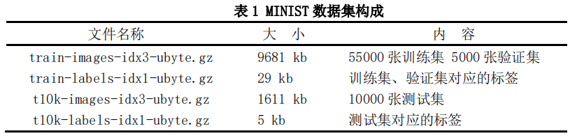
1.1 Data Composition
The MINIST dataset contains a total of70,000A picture of handwritten digits, according to6:1The ratio is divided into training set and test set. The size of the image is28x28, the number of channels is1, each picture is a white text on a black background, the black background is represented by 0 in the tensor, and the white text is represented by a floating point number between 0-1.
The specific data sets and corresponding labels are shown in Table 1.
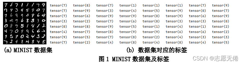
1.2 Data Visualization
Use showdata.py to view the pictures and labels in each batch, as shown in Figure 1.
showdata.py code:
import torch
from torchvision import datasets, transforms
import torchvision
from torch.utils.data import DataLoader
import cv2


# 下载训练集
# transforms.ToTensor将尺寸为[H*W*C]且位于(0,255)的所有PIL图片或者np.uint8的Numpy数组转化为尺寸为(C*H*W)且位于(0.0,1.0)的Tensor
train_dataset = datasets.MNIST(root='.\dataset\mnist',
                train=True,
                transform=transforms.ToTensor(),
                download=True)
# 下载测试集
test_dataset = datasets.MNIST(root='.\dataset\mnist',
               train=False,
               transform=transforms.ToTensor(),
               download=True)

# 装载训练集
train_loader = torch.utils.data.DataLoader(dataset=train_dataset,
                      batch_size=64,
                      shuffle=True)
# 装载测试集
test_loader = torch.utils.data.DataLoader(dataset=test_dataset,
                     batch_size=64,
                     shuffle=True)
# [batch_size,channels,height,weight]
images, labels = next(iter(train_loader))
img = torchvision.utils.make_grid(images)
img = img.numpy().transpose(1, 2, 0)
img = img*255
label=list(labels)

for i in range(len(label)):
    print(label[i],end="\t")
    if (i+1)%8==0:
        print()

cv2.imwrite('1.png', img)
2 Detailed explanation of LeNet and LeNet5 network structure
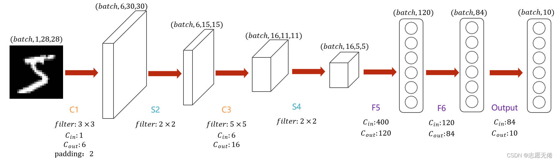
LetNet-5 is a simpler convolutional neural network. The above figure shows its structure: the input two-dimensional image (single channel), first goes through two convolutional layers to the pooling layer, then goes through the fully connected layer, and finally the output layer.
整体上是:input layer->convulational layer->pooling layer->activation function->convulational layer->pooling layer->activation function->convulational layer->fully connect layer->fully connect layer->output layer.
The entire LeNet network includes a total of 7 layers (excluding the input layer),The main difference between LeNet and LeNet5 is the convolution operation in the channel from 6->16。
2.1 Input layer
The input layer (INPUT) is an image of 28x28 pixels, note that the number of channels is 1.
2.2 C1 layer
The C1 layer is a convolution layer, using 6 convolution kernels of 3×3 size, padding=2, stride=1 for convolution, and 630×30Feature map of size: 28+4-3+1=30.
Number of parameters
(3x3+1)x6=60, where 3x3 is the 9 parameters w of the convolution kernel, and 1 is the bias item b.
Connections
60x30x30=54000, where 60 is the number of connections in a single convolution process, 30x30 is the output feature layer, and each pixel is obtained from the previous convolution, that is, a total of 30*30 convolutions have been performed.
2.3 S2 layer
The S2 layer is a downsampling layer, using 6 convolution kernels of 2×2 size for pooling, padding=0, stride=2, and 615×15Size of feature maps: 30/2=15.
Number of parameters
(1+1)x6=12, where the first 1 is the weight w of the largest number in the 2*2 receptive field corresponding to the pooling, and the second 1 is the bias b.
Connections
(2x2+1)x6x15x15= 6750, although only the sum of 2x2 receptive fields is selected, there are also 2x2 connections, 1 is the connection of the bias item, 15x15 is the output feature layer, and each pixel is obtained by the previous convolution. That is, a total of 15x15 convolutions are performed.
2.4 C3 layer
C3 in LeNet is just the convolution shown in the structure diagram, and there is no processing of different feature maps. Here we will not repeat the
different convolution operations of LeNet5 for different feature maps. The following mainly introduces LeNet5
The C3 layer is a convolutional layer, which uses 16 convolution kernels of 5×5 size, padding=0, stride=1 for convolution, and obtains 16 feature maps of 11×11 size: 15-5+1=11.
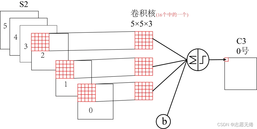
The 16 convolution kernels are not all convolved with the 6 channel layers of S2.
As shown in the figure below, the first six feature maps (0, 1, 2, 3, 4, 5) of C3 are composed of the adjacent three layers of S2. A feature map is used as input, and the corresponding convolution kernel size is: 5x5x3; the
next 6 feature maps (6, 7, 8, 9, 10, 11) are the volumes corresponding to the input of the four adjacent feature maps of S2 The size of the product kernel is: 5x5x4;
the next three feature maps (12, 13, 14) feature maps are taken from the four feature maps interrupted by S2 as input. The corresponding convolution kernel size is: 5x5x4; the last feature
map is No. 15 All (6) feature maps of S2 are used as input, and the corresponding convolution kernel size is: 5x5x6.

It is worth noting that the convolution kernel is 5×5 and has 3 channels, and each channel is different, which is why 5*5 is multiplied by 3, 4, and 6 in the calculation below. This is how multi-channel convolution is calculated.
2.5 S4 layer
The S4 layer is also a downsampling layer like S2, using 16 convolution kernels of 2×2 size for pooling, padding=0, stride=2, and 16 feature maps of 5×5 size are obtained: 11/2=5.
2.6 F5 layer
The C5 layer is a convolutional layer, which uses 120 convolution kernels of 5×5x16 size, padding=0, stride=1 for convolution, and obtains 120 feature maps of 1×1 size: 5-5+1=1. That is, a fully connected layer equivalent to 120 neurons.
It is worth noting that, unlike the C3 layer, the 120 convolution kernels here are convoluted with the 16 channel layers of S4.
Number of parameters
(5516+1)*120=48120。
Connections
4812011=48120。
2.7 F6 layer
F6 is a fully connected layer with a total of 84 neurons, fully connected with C5 layer, that is, each neuron is connected with 120 feature maps of C5 layer. Calculate the dot product between the input vector and the weight vector, plus a bias, and the result is output through the sigmoid function.
2.8 Output layer
The final Output layer is also a fully connected layer, Gaussian Connections, which uses the RBF function (that is, the radial Euclidean distance function) to calculate the Euclidean distance between the input vector and the parameter vector (currently replaced by Softmax).
The Output layer has 10 nodes in total, representing numbers 0 to 9 respectively. Assuming that x is the input of the previous layer and y is the output of RBF, the calculation method of RBF output is:
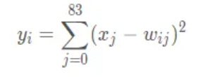
In the above formula, i takes a value from 0 to 9, j takes a value from 0 to 7*12-1, and w is a parameter. The closer the value of RBF output is to 0, the closer to i, that is, the closer to the ASCII code map of i, indicating that the recognition result of the current network input is the character i.
3 LeNet5 source code
import torch
import torch.nn as nn
import torch.nn.functional as F
import numpy as np
# 卷积层使用 torch.nn.Conv2d
# 激活层使用 torch.nn.ReLU
# 池化层使用 torch.nn.MaxPool2d
# 全连接层使用 torch.nn.Linear

class LeNet(nn.Module):
  def __init__(self,num_classes=10):
    super(LeNet, self).__init__()
    self.conv1 = nn.Sequential(nn.Conv2d(in_channels=1, out_channels=6,kernel_size=3,stride=1,padding= 2),
                  nn.ReLU(),
                  nn.MaxPool2d(kernel_size=2))

    # 第一组卷积核
    self.conv2_1_1=nn.Sequential(nn.Conv2d(in_channels=3,out_channels=1,kernel_size=5)
                                 ,nn.ReLU())
    self.conv2_1_2=nn.Sequential(nn.Conv2d(in_channels=4,out_channels=1,kernel_size=5)
                                 ,nn.ReLU())
    self.conv2_1_3=nn.Sequential(nn.Conv2d(in_channels=4,out_channels=1,kernel_size=5)
                                 ,nn.ReLU())
    self.conv2_1_4=nn.Sequential(nn.Conv2d(in_channels=6,out_channels=1,kernel_size=5))

    self.conv3=nn.Sequential(nn.ReLU(),
                  nn.MaxPool2d(kernel_size=2))

    self.fc1 = nn.Sequential(nn.Linear(16 * 5 * 5, 120),
                 #数据归一化处理
                 nn.BatchNorm1d(120),
                 nn.ReLU())

    self.fc2 = nn.Sequential(
      nn.Linear(120, 84),
      nn.BatchNorm1d(84),
      nn.ReLU(),
      nn.Linear(84, num_classes))
    # 最后的结果一定要变为 10,因为数字的选项是 0 ~ 9

  def forward(self, x):
    # print(x.shape)
    x = self.conv1(x)
    # print(x.shape)
    x_0,x_1,x_2,x_3,x_4,x_5=x.split(1,dim=1)
    # print(x_0.shape)
    out_1_0=self.conv2_1_1(torch.cat((x_0,x_1,x_2),1))
    out_1_1=self.conv2_1_1(torch.cat((x_1,x_2,x_3),1))
    out_1_2 = self.conv2_1_1(torch.cat((x_2, x_3, x_4), 1))
    out_1_3 = self.conv2_1_1(torch.cat((x_3, x_4, x_5), 1))
    out_1_4 = self.conv2_1_1(torch.cat((x_4, x_5, x_0), 1))
    out_1_5 = self.conv2_1_1(torch.cat((x_5, x_0, x_1), 1))
    out_1=torch.cat((out_1_0,out_1_1,out_1_2,out_1_3,out_1_4,out_1_5),1)
    # print("第一组操作结束时维度:",out_1.shape)

    out_2_0=self.conv2_1_2(torch.cat((x_0,x_1,x_2,x_3),1))
    out_2_1 = self.conv2_1_2(torch.cat((x_1, x_2, x_3, x_4), 1))
    out_2_2 = self.conv2_1_2(torch.cat((x_2, x_3, x_4, x_5), 1))
    out_2_3 = self.conv2_1_2(torch.cat((x_3, x_4, x_5, x_0), 1))
    out_2_4 = self.conv2_1_2(torch.cat((x_4, x_5, x_0, x_1), 1))
    out_2_5 = self.conv2_1_2(torch.cat((x_5, x_0, x_1, x_2), 1))
    out_2=torch.cat((out_2_0,out_2_1,out_2_2,out_2_3,out_2_4,out_2_5),1)
    # print("第二组操作结束时维度:", out_2.shape)

    out_3_0=self.conv2_1_3(torch.cat((x_0,x_1,x_3,x_4),1))
    out_3_1 = self.conv2_1_3(torch.cat((x_1, x_2, x_4, x_5), 1))
    out_3_2 = self.conv2_1_3(torch.cat((x_2, x_3, x_5, x_0), 1))
    out_3=torch.cat((out_3_0,out_3_1,out_3_2),1)
    # print("第三组操作结束时维度:", out_3.shape)

    out_4=self.conv2_1_4(x)
    # print("第四组操作结束时维度:", out_4.shape)

    x=torch.cat((out_1,out_2,out_3,out_4),1)
    # print(x.shape)

    x=self.conv3(x)
    # print(x.shape)
    x = x.view(x.size()[0], -1)
    # print(x.shape)
    x = self.fc1(x)
    # print(x.shape)
    x = self.fc2(x)
    # print(x.shape)
    return x
4 training code
import time
import os
from tqdm import tqdm
import logging
from models import LeNet
from torchvision import datasets, transforms
from tensorboardX import SummaryWriter
import numpy as np
import torch
import torch.nn as nn
from torch.utils.data import DataLoader
from torchvision import transforms
import warnings
# 忽略Warning
warnings.filterwarnings('ignore')

os.environ['CUDA_VISIBLE_DEVICES'] = '0'
Batch_size=8
Save_path="saved/"
Save_model="LeNet"
Summary_path=r'.\runs\LeNet5'
Num_classes=10
if not os.path.exists(Summary_path):
    os.mkdir(Summary_path)
writer = SummaryWriter(log_dir=Summary_path, purge_step=0)

def train():

    # train配置
    device = torch.device('cuda:0')
    model = LeNet(num_classes=Num_classes)
    # model = nn.DataParallel(model, device_ids=[0, 1])
    model.to(device)

    logger = initLogger("Mnist_LeNet")

    # loss
    criterion = nn.CrossEntropyLoss()

    # train data
    train_dataset = datasets.MNIST(root='.\mnist',
                    train=True,
                    transform=transforms.ToTensor(),# 数据类型预处理,变成张量并归一化(/255)
                    download=True)
    # 下载测试集
    val_dataset = datasets.MNIST(root='.\mnist',
                train=False,
                transform=transforms.ToTensor(),
                download=True)

    # 装载训练集
    train_loader = torch.utils.data.DataLoader(dataset=train_dataset,
                        batch_size=Batch_size,
                        shuffle=True)
    # 装载验证集
    val_loader = torch.utils.data.DataLoader(dataset=val_dataset,
                        batch_size=Batch_size,
                        shuffle=True)


    # optimizer
    optimizer = torch.optim.Adam(model.parameters(), lr=0.0001, weight_decay=0.0001)
    #最优val准确率,根据这个保存模型
    val_max_OA = 0.0
    for epoch in range(100):
        # lr
        model.train()
        loss_sum = 0.0
        correct_sum = 0.0
        total=0
        # train_loader为可迭代对象,ncols为自定义的进度条长度
        tbar = tqdm(train_loader, ncols=120)
        for batch_idx, (data, target) in enumerate(tbar):
            data=data.cuda()
            target=target.cuda()
            # data, target = data.to(device), target.to(device)
            optimizer.zero_grad()# 清除梯度
            output = model(data)
            loss = criterion(output, target)
            loss_sum += loss.item()

            loss.backward()# 反向传播,计算张量的梯度
            optimizer.step()# 根据梯度更新网络参数
            # torch.max(x,dim=?) dim=0时返回每一列中最大值的那个元素的值和索引,dim=1时返回每一行中最大值的那个元素值和索引
            # 值无用,需要的是索引,也即0-9的标签,不用转化正好时标签
            # out输出10个类各自的概率,所以需要从每一条数据中取出最大的
            _,predicted=torch.max(output,1)
            correct_sum += (predicted == target).sum()
            total += Batch_size
            oa=correct_sum.item()/total*1.0
            # 轮次、损失总值、正确率
            tbar.set_description('TRAIN ({}) | Loss: {:.5f} | OA {:.5f} |'.format(
                epoch, loss_sum/((batch_idx+1)*Batch_size),oa))

        # 使用TensorBoard记录各指标曲线
        writer.add_scalar('train_loss', loss_sum / ((batch_idx + 1) * Batch_size), epoch)
        writer.add_scalar('train_oa', oa, epoch)

        # 每一轮次结束后记录运行日志
        logger.info('TRAIN ({}) | Loss: {:.5f} | OA {:.5f}'.format(
            epoch, loss_sum/((batch_idx+1)*Batch_size),oa))


        # val

        model.eval()
        loss_sum = 0.0
        correct_sum = 0.0
        total=0
        tbar = tqdm(val_loader, ncols=120)
        class_precision=np.zeros(Num_classes)
        class_recall=np.zeros(Num_classes)
        class_f1=np.zeros(Num_classes)
        # val_list=[]

        # data, target = data.to(device), target.to(device)
        with torch.no_grad():
            #混淆矩阵
            conf_matrix_val = np.zeros((Num_classes,Num_classes))
            for batch_idx, (data, target) in enumerate(tbar):
                data=data.cuda()
                target=target.cuda()
                output = model(data)
                loss = criterion(output, target)
                loss_sum += loss.item()

                _,predicted=torch.max(output,1)
                correct_sum += (predicted == target).sum()
                total += Batch_size

                oa=correct_sum.item()/total*1.0

                c_predict=predicted.cpu().numpy()
                c_target=target.cpu().numpy()


                # 预测值为行标签、真值为列标签,类似两标签下的混淆矩阵
                '''
                        预测值
                真值  正      负
                正   TP      FN
                负   FN      TN
                '''
                for i in range(len(c_predict)):
                    conf_matrix_val[c_target[i],c_predict[i]] += 1
                for i in range(Num_classes):
                    #每一类的precision
                    class_precision[i]=1.0*conf_matrix_val[i,i]/conf_matrix_val[:,i].sum()
                    #每一类的recall
                    class_recall[i]=1.0*conf_matrix_val[i,i]/conf_matrix_val[i].sum()
                    #每一类的f1
                    class_f1[i]=(2.0*class_precision[i]*class_recall[i])/(class_precision[i]+class_recall[i])

                tbar.set_description('VAL ({}) | Loss: {:.5f} | OA {:.5f} '.format(
                    epoch, loss_sum / ((batch_idx + 1) * Batch_size),
                    oa))
            # 保存最优oa对应的模型
            if oa > val_max_OA:
                val_max_OA = oa
                best_epoch =np.zeros(2)
                best_epoch[0]=epoch
                best_epoch[1]=conf_matrix_val.sum()
                if os.path.exists(Save_path) is False:
                    os.mkdir(Save_path)
                torch.save(model.state_dict(), os.path.join(Save_path, Save_model+'.pth'))
                np.savetxt(os.path.join(Save_path,  Save_model+'_conf_matrix_val.txt'),conf_matrix_val,fmt="%d")
                np.savetxt(os.path.join(Save_path, Save_model+'_best_epoch.txt'),best_epoch,fmt="%d")

        writer.add_scalar('val_loss', loss_sum / ((batch_idx + 1) * Batch_size), epoch)
        writer.add_scalar('val_oa', oa, epoch)
        writer.add_scalar('Avarage_percision', class_precision.sum()/10, epoch)
        writer.add_scalar('Avarge_recall', class_recall.sum()/10, epoch)
        writer.add_scalar('Avarage_F1', class_f1.sum()/10, epoch)

        logger.info('VAL ({}) | Loss: {:.5f} | OA {:.5f} |class_precision {}| class_recall {} | class_f1 {}|'.format(
            epoch, loss_sum / ((batch_idx + 1) * Batch_size),
            oa,toString(class_precision),toString(class_recall),toString(class_f1)))

def toString(IOU):
    result = '{'
    for i, num in enumerate(IOU):
        result += str(i) + ': ' + '{:.4f}, '.format(num)

    result += '}'
    return result

def initLogger(model_name):
    # 初始化log
    logger = logging.getLogger()
    logger.setLevel(logging.INFO)

    rq = time.strftime('%Y%m%d%H%M', time.localtime(time.time()))
    log_path = r'logs'
    if not os.path.exists(log_path):
        os.mkdir(log_path)
    log_name = os.path.join(log_path, model_name + '_' + rq + '.log')
    logfile = log_name
    fh = logging.FileHandler(logfile, mode='w')
    fh.setLevel(logging.INFO)

    formatter = logging.Formatter("%(asctime)s - %(filename)s[line:%(lineno)d] - %(levelname)s: %(message)s")
    fh.setFormatter(formatter)
    logger.addHandler(fh)

    return logger

if __name__ == '__main__':
    train()