Table of contents
foreword
Recently, I am learning data structure and algorithm, so write a note to record it.
1. Algorithm
1. What is a hash table?
Let’s start with an appetizer. We often hear hash, so let’s take a brief look at what hash is, and we will introduce it in detail later.
Hash Table (Hash Table), also known as hash map or dictionary, is a common data structure used to store key-value pairs (key-value pairs). It maps keys to buckets or slots by using a hash function to enable fast insertion, lookup, and deletion. The core idea of a hash table is to use the hash value of the key as an index to access and store the value.
2. What is time complexity?
Time complexity is the relationship between the algorithm running time and the input scale, which is used to measure the efficiency of the algorithm. It describes the number of operations required for an algorithm to perform, usually expressed in Big O notation (O). When calculating time complexity, the main focus is on the part of the code that is executed the most in the algorithm.
- Constant time complexity (O(1)): The execution time of the algorithm is fixed and constant regardless of the size of the input. For example, operations such as simple assignment statements and accessing array elements have constant time complexity.
- Linear time complexity (O(n)): The execution time of the algorithm is linear in the size of the input. For example, the time complexity of traversing an array containing n elements is O(n).
- Logarithmic time complexity (O(log n)): The logarithmic relationship between the execution time of the algorithm and the input size. Usually occurs when using algorithms such as divide and conquer or binary search. For example, the time complexity of binary search is O(log n).
- Quadratic time complexity (O(n 2)), cubic time complexity (O(n 3)), etc.: The relationship between the execution time of the algorithm and the square, cube, etc. of the input scale. For example, nested loop operations often result in quadratic time complexity.
- Exponential time complexity (O(2^n)): The exponential relationship between the execution time of the algorithm and the input size. Usually occurs when using an exponential algorithm such as exhaustive search, because its execution time grows dramatically with the size of the input.
Quickly judge algorithm complexity (applicable to most simple cases)
- Determine the problem size n
- Cyclic halving process - logn
- The cycle of k layer about n > nkn^{k}nk
- Complicated situations: Judgment based on the algorithm execution process
3. Space complexity
Space complexity: the formula used to evaluate the memory footprint of the algorithm, the expression of space complexity is exactly the same as the time complexity
- The algorithm uses several variables: O(1)
- The algorithm uses a one-dimensional list of length n: O(n)
- The algorithm uses a two-dimensional list of m rows and n columns: O(mn)
- space for time
4. Recursion
Two constraints: call itself, end condition
def fun1(x):
    if x > 0:
        print(x)
        fun1(x - 1)


def fun2(x):
    if x > 0:
        fun1(x - 1)
        print(x)


if __name__ == "__main__":
    fun1(3)
    fun2(3)
optput:
3
2
1
1
2
3
Why is the next one 1,2,3? Look at the picture below: the execution of the function is from top to bottom, the one on the left is printed after recursion, and the one on the right is printed after recursion.

Look at the problem of the Tower of Hanoi:
def han(n, a, b, c):

    if n > 0:
        han(n - 1, a, c, b)
        print("moving from %s to %s" % (a, c))
        han(n - 1, b, a, c)


if __name__ == "__main__":
    han(10 , "A", "B", "C")
4. Find
Search: Among some data elements, the process of finding the same data element as a given keyword by a certain method.
- List lookup (linear table lookup): Find the specified element from the list
- Input: list, element to be found
- Output: element subscript (generally returns None or -1 when no element is found)
- Built-in list lookup functions:
index()
4.1, sequential search
for loop
def linear_search(data_set, value):
    for i in range(len(data_set)):
        if data_set[i] == value:
            return i
    return
4.2. Binary search
It is required that the list must be an ordered list, sorted first, left and right record the variables on both sides, find the middle element mid, and update left, right, mid.
The following code is assumed to have been sorted. Sorting can be done directly with sorted().
def binary_search(data_list, value):
    left = 0
    right = len(data_list)

    while left <= right:
        mid = (left + right) //2
        if data_list[mid] == value:
            return mid
        elif data_list[mid] > value:
            right = mid -1
        else:
            left = mid + 1
5. Sort
Sort: Resizes a set of "unordered" record sequences into an "ordered" record sequence.
List sorting: turn an unordered list into an ordered list
- input: list
- output: ordered list
- ascending and descending
- Built-in sort functions:
sorted()
5.1. Bubble sort
A large number sinks or floats, and compares them pairwise for exchange.

def bubble_sort(array):
    for i in range(len(array)):
        for j in range(len(array) - 1 - i):
            if array[j] > array[j + 1]:
                array[j], array[j + 1] = array[j + 1], array[j]
    return array
The above code has a shortcoming. If a list does not need to go through all n-1 times, can it be improved?
def bubble_sort(array):
    for i in range(len(array)):
        exchange = False
        for j in range(len(array) - 1 - i):
            if array[j] > array[j + 1]:
                array[j], array[j + 1] = array[j + 1], array[j]
                exchange = True
    return array
5.2. Selection sort
Choose the smallest or largest and put them in front.

def select_sort(li):
    for i in range(len(li)-1):
        min_loc = i
        for j in range(i+1, len(li)):
            if li[j] < li[min_loc]:
                min_loc = j
            li[i], li[min_loc] = li[min_loc], li[i]
5.3. Insertion sort
When drawing cards, sort the cards according to the insertion method.

def insertion_sort(arr):
    n = len(arr)
    for i in range(1, n):
        key = arr[i]  # 待插入的元素
        j = i - 1  # 已排序序列的最后一个元素的索引

        # 将比待插入元素大的元素向右移动
        while j >= 0 and arr[j] > key:
            arr[j + 1] = arr[j]
            j -= 1

        # 插入待排序元素到正确位置
        arr[j + 1] = key
Summarize:
Bubble sorting, selection sorting, and insertion sorting are far lower sorting, and the complexity is O ( n 2 ) O(n^{2})O ( n2 ), the implementation is simple, the disadvantage is
5.4. Quick Sort
Quick sort: fast
quick sort ideas (somewhat similar to dichotomy)

- Take an element p ( the first element ), and make the element p return (put it where it should be);
- The list is divided into two parts by p, the left side is smaller than p, and the right side is larger than p;
- Recursively complete the sort
def partition(li, left, right):
    tmp = li[left]
    while left < right:
        while left < right and li[right] >= tmp:  # 从右面找比tmp小的数
            # 往左走一步
            right -= 1
        li[left] = li[right]
        # 把右边的值写到左边空位上
        while left < right and li[left] <= tmp:
            left += 1
        li[right] = li[left]
    # 把左边的值写到右边空位上
    li[left] = tmp  # 把tmp归位
    return left


def quick_sort(data, left, right):
    if left < right:
        mid = partition(data, left, right)
        quick_sort(data, left, mid - 1)
        quick_sort(data, mid + 1, right)
    return data
Time complexity of quicksort O ( nlogn ) O(nlogn)O ( n l o g n )
Disadvantages: Recursion, there will be the worst case (the initial test list is the complexity of reverse order orO ( n 2 ) ) O(n^{2}))O ( n2 )), shuffling the list can alleviate this from happening.
5.5. Heap sort
5.5.1. Trees
To heap sort, you must first know what a tree is.

A heap is a special kind of complete binary tree.
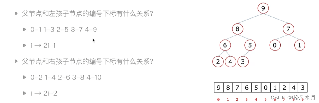
How is a binary tree implemented in a computer, that is, how is it stored?
There are two ways: chained storage (linked list will be introduced later), and sequential storage .
Sequential storage is processed in a list.
Let's take a complete binary tree as an example:
5.5.2. Heap
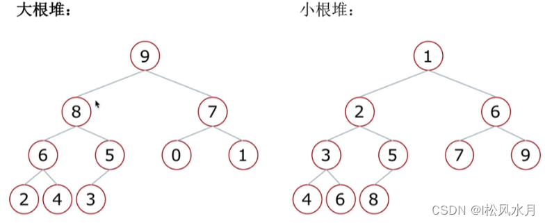
Heap: A special complete binary tree structure
Two structures:
- Large root heap: a complete binary tree, satisfying that any node is larger than its child nodes
- Small root heap: a complete binary tree, satisfying that any node is smaller than its child nodes
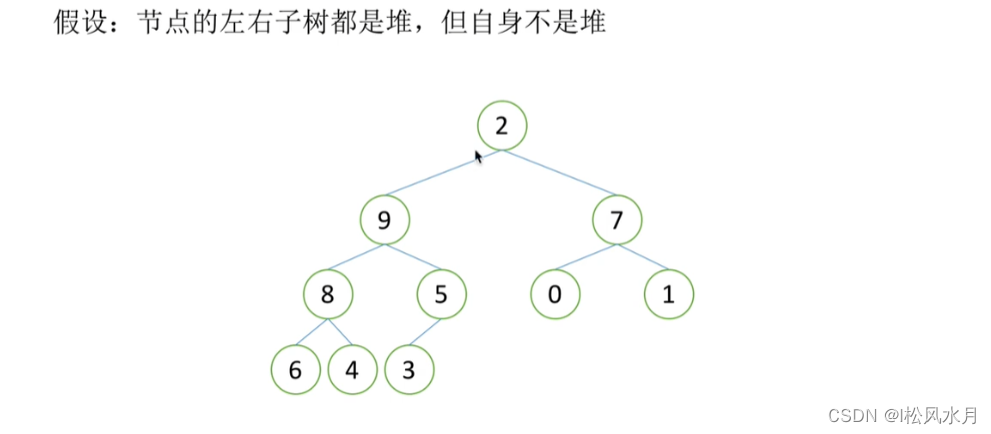
The heap has a downscaling type:
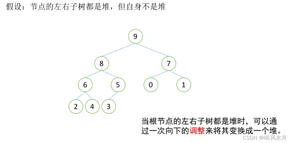
Assuming that the left and right subtrees of the root node are both heaps, but the root node does not satisfy the nature of the heap, it can be turned into a heap by a downward adjustment
adjusted:
How is the heap constructed?
From the very beginning, it will be adjusted level by level, and the countryside will surround the cities.
process:
- Create a heap, take Dagen Heap as an example
- Get the top element of the heap, which is the largest element
- Remove the top of the heap, put the last element of the heap on the top of the heap, at which point the heap can be reordered with only one downward adjustment
- The top element of the heap is the second largest element
- Repeat step 3 until the heap becomes empty
The core of heap sorting is to build a heap + a downward adjustment. If you want to build a heap, the core is to make the lower levels in order first. As long as the lower levels are satisfied with the heap, you can build a complete heap through one downward adjustment step by step, and finally you can Traverse the top elements one by one to sort the entire list
# 只是一次调整堆
def sift(li, low, high):
    """
    :param li: 列表
    :param low: 堆的根节点位置
    :param high: 堆的最后一个元素的位置
    :return:
    """
    i = low  # i最开始指向根节点
    j = 2 * i + 1  # 开始是左孩子
    tmp = li[low]  # 把堆顶存起来
    while j <= high:  # 只要j位置有数
        if j + 1 <= high and li[j + 1] > li[j]:  # 如果右孩子有并且比较大
            j = j + 1  # 指向右孩子
        if li[j] > tmp:
            li[i] = li[j]
            i = j  # 往下看一层
            j = 2 * i + 1
        else:  # tmp更大,把tmp放到i的位置上li[i] = tmp#把tmp放到某一级领导位置上break
            li[i] = tmp  # 把tmp放到叶子节点上
            break
    else:
        li[i] = tmp


def heap_sort(li):
    n = len(li)
    # 从最下面的左边的叶子结点开始调整建堆
    for i in range((n - 2) // 2, -1, -1):
        sift(li, i, n - 1)
    # print(li)
    # 排序
    for i in range(n - 1, -1, -1):
        li[0], li[i] = li[i], li[0]
        sift(li, 0, i - 1)
    return li
Time complexity: O ( nlogn ) O(nlogn)O(nlogn)
Heap built-in modules:
- heapify(x)
- heappush(heap,item)
- heappop(heap)
Now there are n numbers, design an algorithm to get the top k largest numbers. (k<n)
solution ideas:
- Slicing after sorting: O(nlogn)
- Sort LowB trios: O(kn)
- Heap sorting idea: O(nlogk), small root heap implementation
Heap sorting implementation method: two sets of animations to demonstrate.


def sift(li, low, high):
    """
    :param li: 列表
    :param low: 堆的根节点位置
    :param high: 堆的最后一个元素的位置
    :return:
    """
    i = low  # i最开始指向根节点
    j = 2 * i + 1  # 开始是左孩子
    tmp = li[low]  # 把堆顶存起来
    while j <= high:  # 只要j位置有数
        if j + 1 <= high and li[j + 1] < li[j]:  # 如果右孩子有并且比较大
            j = j + 1  # 指向右孩子
        if li[j] < tmp:
            li[i] = li[j]
            i = j  # 往下看一层
            j = 2 * i + 1
        else:  # tmp更大,把tmp放到i的位置上li[i] = tmp#把tmp放到某一级领导位置上break
            li[i] = tmp  # 把tmp放到叶子节点上
            break
    else:
        li[i] = tmp

def topk(li, k):
	# 列表前k个取出来建堆
    heap = li[0:k]
    for i in range((k - 2) // 2, -1, -1):
        sift(heap, i, k - 1)
    # 建堆
    for i in range(k, len(li)-1):
        if li[i] > heap[0]:
            heap[0] = li[i]
            sift(heap, 0, k-1)
    # 遍历
    for i in range(k - 1, -1, -1):
        heap[0], heap[i] = heap[i], heap[0]
        sift(heap, 0, i - 1)
    # 输出
    return heap
5.6. Merge sort
A list can be divided into two parts, both sides are sorted. likelist = [1, 2, 3, 4, 2, 3, 7, 9]
def merge(li, low, mid, high):
    i = low
    j = mid + 1
    ltmp = []
    while i <= mid and j <= high:
        if li[i] < li[j]:
            ltmp.append(li[i])
            i += 1
        else:
            ltmp.append(li[j])
            j += 1
    while i <= mid:
        ltmp.append((li[i]))
        i += 1
    while j <= high:
        ltmp.append(li[j])
        j += 1
    li[low:high + 1] = ltmp
    return li
In actual use, the list is not divided into two and sorted, how to deal with it?
- Decomposition: divide the list into smaller and smaller ones until it is divided into one element
- Termination condition: An element is ordered.
- Merge: Merge two sorted lists, the lists get bigger and bigger.
Merge diagram:


How should the complete code be implemented?
def merge(li, low, mid, high):
    i = low
    j = mid + 1
    ltmp = []
    while i <= mid and j <= high:
        if li[i] < li[j]:
            ltmp.append(li[i])
            i += 1
        else:
            ltmp.append(li[j])
            j += 1
    ltmp.extend(li[i:mid + 1])
    ltmp.extend(li[j:high + 1])
    li[low:high + 1] = ltmp


def merge_sort(li, low, high):
    if low < high:
        mid = (low + high) // 2
        merge_sort(li, low, mid)
        merge_sort(li, mid + 1, high)
        merge(li, low, mid, high)
    return li
Python's built-in sorted sorting method is optimized based on merge sort.
Time complexity: O ( nlogn ) O(nlogn)O ( n log n )
Summary:
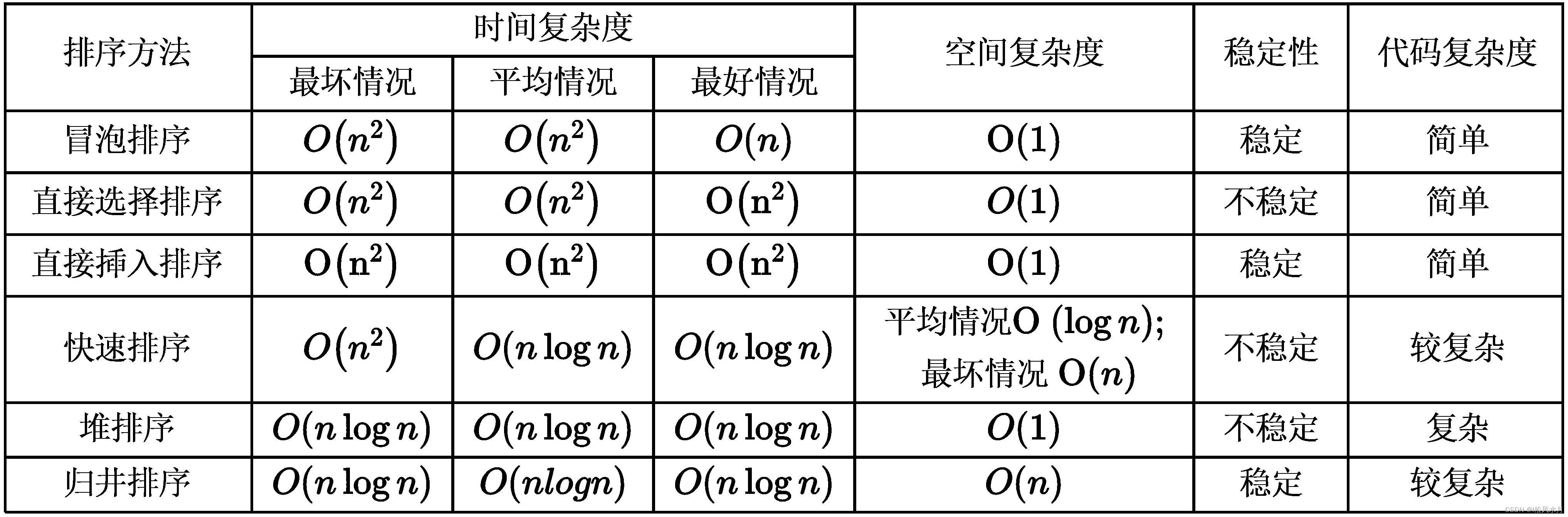 Those who move one by one are stable, and those who are not changed one by one are unstable .
5.7. Hill sort
Shell Sort is a grouping insertion sorting algorithm, an improved version of the insertion sorting algorithm, and a very stable algorithm.
- First take an integer d=n/2, divide the elements into d groups, the distance between each group of adjacent elements is d, and perform direct insertion sorting in each group;
- Take the second integer d,=d,/2, and repeat the above grouping sorting process until d;=1, that is, all elements are directly inserted into the same group.
- Each pass of Hill sorting does not make some elements in order, but makes the overall data closer and closer to order; the last sort makes all data in order.


def insert_sort_gap(li, gap):
    for i in range(gap, len(li)):
        tmp = li[i]
        j = i -gap
        while j >= 0 and li[j] > tmp:
            li[j+gap] = li[j]
            j -= gap
        li[j+gap] = tmp

def shell_sort(li):
    d = len(li) // 2
    while d >= 1:
        insert_sort_gap(li, d)
        d //= 2
    return li
5.8. Counting sort
Count the number of occurrences of a number directly.

def count_sort(li, max_count):
    count = [0 for _ in range(max_count + 1)]
    for val in li:
        count[val] += 1
    li.clear()
    for index, val in enumerate(count):
        for i in range(val):
            li.append(index)

    return li


li = [3, 2, 6, 1, 7, 9, 6, 8]
# 注意这里传的是最大值
result = count_sort(li, max(li))
print(result)
print(sorted(li))
When encountering a dictionary, it can be placed in a list.
Disadvantages: The list is short, and it is not very friendly when the value is large. How to solve it, lead to bucket sorting.
5.9. Bucket Sort
An improvement to counting sort, which puts a range of elements together. It's not very important, just know the principle code and write it out.
Bucket Sort:
- First divide the elements into different buckets, and then sort the elements in each bucket 29 25 3 49 9 37 21 43

def bucket_sort(li, n, max_num):
    # 创建桶
    buckets = [[] for _ in range(n)]
    for var in li:
        # 去最小值是因为当值为最后一位的时候数组下标会越界,如10000分为100组,10000的时候数应该放在99下标的数组中,而不是100
        i = min(var // (max_num // n), n - 1)
        buckets[i].append(var)
        # 装进桶的同时进行排序,只需要给前面一个数比较看谁大就行了,保证了每个桶的数按照顺序放入
        for j in range(len(buckets[i]) - 1, 0, -1):
            if buckets[i][j] < buckets[i][j-1]:
                buckets[i][j], buckets[i][j - 1] = buckets[i][j - 1], buckets[i][j]
            else:
                break
    sorted_li = []
    for buc in buckets:
        sorted_li.extend(buc)
    return sorted_li
The performance of bucket sort depends on the distribution of the data. That is, different bucketing strategies need to be adopted when sorting different data.
- Average case time complexity: O(n+k)
- Worst case time complexity: O(n2k)
- Space Complexity: O(nk)
5.10. Radix sort
The improvement of bucket sorting is to sort according to single digit first, output, and then sort according to 10 digits.

def radix_sort(li):
    max_num = max(li)
    # 求最大数的位数
    it = 0
    while 10 ** it <= max_num:
        # 固定10个桶
        buckets = [[] for _ in range(10)]
        for var in li:
            # 从前往后依次取数,如987,->7,8,9
            digit = (var // 10 ** it) % 10
            buckets[digit].append(var)
        # 按照对应位数粪桶完成
        li.clear()
        for buc in buckets:
            li.extend(buc)
        it += 1
    return li
Time complexity: O ( kn ) O(kn)O ( kn ) , k is a base 10 number

2. Data structure
Data structures can be roughly divided into three categories: linear structures, tree structures, and graph structures.
2.1. List/Array
Lists (or arrays in other languages) are a primitive data type.
Arrays are different from lists in two ways: the array elements must be the same and have a fixed length, which is not required in Python. So how does the list in python realize that the elements can be different and the length is fixed? The address stored in the python list is no longer a value. Putting the address of the element in the list is a pointer in C. When the length is not enough, the list will open up by itself.
some problems with the list
- How are the elements in the list stored?
- Basic operations of lists: search by index, insert elements, delete elements...
- What is the time complexity of these operations?
- How are Python lists implemented?
Some operations of the list can refer to: A detailed explanation of list, tuple, dictionary, collection, generator, iterator, iterable object, zip, enumerate .
2.2. Stack
Stack (Stack) is a collection of data, which can be understood as a list that can only be inserted or deleted at one end.
- The characteristics of the stack: the concept of first out of the stack: the top of the stack, the bottom of the stack
- The basic operations of the stack: Push (push): push Pop out: pop Take the top of the stack: gettop
- The stack can be realized by using the general list structure: push into the stack: li.append; pop out of the stack: li.pop; take the top of the stack: li[-1]
A simple implementation of a stack:
class Stack:
    def __init__(self):
        self.stack = []

    def push(self, element):
        self.stack.append(element)

    def pop(self):
        return self.stack.pop()

    def get_top(self):
        if len(self.stack) > 0:
            return self.stack[-1]
        else:
            return None

stack = Stack()
stack.push(1)
stack.push(2)
stack.push(3)
print(stack.pop())
Application: Where can the stack be used?
See a parenthesis matching problem. Check that the parentheses are spelled correctly.
class Stack:
    def __init__(self):
        self.stack = []

    def push(self, element):
        self.stack.append(element)

    def pop(self):
        return self.stack.pop()

    def get_top(self):
        if len(self.stack) > 0:
            return self.stack[-1]
        else:
            return None

    def is_empty(self):
        return len(self.stack) == 0


def brace_match(s):
    match = {

    "}": "{", "]": "[", ")": "("}
    stack = Stack()
    for ch in s:
        if ch in {

    "(", "{", "["}:
            stack.push(ch)
        else:
            if stack.is_empty():
                return False
            elif stack.get_top() == match[ch]:
                stack.pop()
            else:
                return False
    if stack.is_empty():
        return True
    else:
        False


print(brace_match("[][][]{}{}({})"))
print(brace_match("[{]}"))
2.3. Queue
A queue (Queue) is a collection of data that only allows insertion at one end of the list and deletion at the other end. The end of the insertion is called the rear of the queue, the end of the insertion action is called entering the queue or entering the queue for deletion is called the front of the queue, and the deletion action is called the dequeue. The nature of the queue: First-in-first-
out ,First-out)
Queue implementation method: Ring queue
Ring queue: When the tail pointer is moved front == Maxsize - 1, it will automatically reach 0.
The queue pointer advances 1: front =(front +1)% MaxSize
The tail pointer advances 1: rear =(rear + 1)% MaxSize
Empty conditions: rear == front
Full conditions:(rear +1)% MaxSize == front

Implement a circular queue yourself:
class Queue:
    def __init__(self, size=100):
        self.queue = [0 for _ in range(size)]
        self.size = size
        # 队首指针
        self.rear = 0
        # 队尾指针
        self.front = 0

    def push(self, element):
        if not self.is_filled():
            self.rear = (self.rear + 1) % self.size
            self.queue[self.rear] = element
        else:
            raise IndexError("队列已满")

    def pop(self):
        if not self.is_empty():
            self.front = (self.front + 1) % self.size
            return self.queue[self.front]
        else:
            raise IndexError("队列为空")

    def is_empty(self):
        return self.rear == self.front

    def is_filled(self):
        return (self.rear + 1) % self.size == self.front

q = Queue(5)
for i in range(4):
    q.push(i)
print(q.pop())
q.push(4)
The above queue is a one-way queue, which can only enter first in first out, and cannot enter and exit in both directions. So there is a two-way queue, a queue that can enter and exit at both ends of the two-way queue.
Python built-in queue module:
The queue package in python is not a queue package, but a package that guarantees thread safety. The queue package from collections import dequerepresents a two-way queue by introducing deque, collectionsin which some data structure packages are stored.
使用方法: from collections import deque
# 创建的是个双向队列
创建队列: queue = deque()
# 单向队列
进队: append() # 队尾进队
出队: popleft() # 队首出队
# 双向队列时的操作,一般用的不多
双向队列队首进队: appendleft()
双向队列队尾出队: pop()
from collections import deque
# 队满自动出列
q = deque([1, 2, 3, 4, 5], 3)
print(q)
output:
deque([3, 4, 5], maxlen=3)
Let's look at another question about using a queue to implement the tell function of Linux:
# file.txt文件
1223
rwqer
qewf
vdsg
q3wr
xczv
24141fswf
wqeq
fsgfd
from collections import deque
# 用队列实现linux的tell函数
def tell(n):
    with open("file.txt", "r") as f:
        # deque可以接收一个可迭代对象,deque会自动迭代文件对象f并将其行存储在队列中。
        q = deque(f, n)
        return q
for line in tell(5):
    print(line, end="")
output:
q3wr
xczv
24141fswf
wqeq
fsgfd
What if the above question is changed to the first few lines? Direct user for loop to traverse the first few on the line.
Let's look at the maze problem again:
# 0表示路,1表示墙
maze = [
    [1, 1, 1, 1, 1, 1, 1, 1, 1, 1],
    [1, 0, 0, 1, 0, 0, 0, 1, 0, 1],
    [1, 0, 0, 1, 0, 0, 0, 1, 0, 1],
    [1, 0, 0, 0, 0, 1, 1, 0, 0, 1],
    [1, 0, 1, 1, 1, 0, 0, 0, 0, 0],
    [1, 0, 0, 0, 0, 0, 1, 1, 0, 1],
    [1, 1, 1, 0, 1, 1, 1, 1, 1, 0],
    [1, 1, 1, 0, 0, 1, 0, 1, 0, 1],
    [1, 0, 0, 1, 0, 0, 0, 0, 0, 1],
    [1, 1, 0, 0, 0, 1, 1, 1, 1, 1]
]

dirs = [
    lambda x, y: (x + 1, y),
    lambda x, y: (x - 1, y),
    lambda x, y: (x, y - 1),
    lambda x, y: (x, y + 1),
]

def maze_path(x1, y1, x2, y2):
    stack = []
    stack.append((x1, y1))
    # 栈不空时循环,栈空表示没路可走了
    while len(stack) > 0:
        curNode = stack[-1]
        if curNode[0] == x2 and curNode[1] == y2:
            for p in stack:
                print(p)
            return True
        # 遍历四个方向
        for dir in dirs:
            nextNode = dir(curNode[0], curNode[1])
            # 检查下一个节点是否越界
            if nextNode[0] < 0 or nextNode[0] >= len(maze) or nextNode[1] < 0 or nextNode[1] >= len(maze[0]):
                continue
            # 如果下一个节点能走且未访问过
            if maze[nextNode[0]][nextNode[1]] == 0:
                stack.append(nextNode)
                # 标记已经走过
                maze[nextNode[0]][nextNode[1]] = 2
                break
        else:
            # 四个方向都无法前进,回溯
            stack.pop()
    else:
        print("没有路")
        return False

maze_path(1, 1, 8, 8)
output:
(1, 1)
(2, 1)
(3, 1)
(4, 1)
(5, 1)
(5, 2)
(5, 3)
(6, 3)
(7, 3)
(7, 4)
(8, 4)
(8, 5)
(8, 6)
(8, 7)
(8, 8)
The linked list queue can solve the fixed length problem of the ring queue.
2.4. Linked list
A linked list is a collection of elements composed of a series of nodes. Each node consists of two parts, the data field item and the pointer next to the next node. Through the interconnection between nodes, a linked list is finally concatenated.
See a simple linked list demo
class Node:
    def __init__(self, item):
        self.item = item
        self.next = None

a = Node(1)
b = Node(2)
c = Node(3)

a.next = b
b.next = c

print(a.next.next.item)
How to create a linked list? Head plugging method, tail plugging method.
class Node:
    def __init__(self, item):
        self.item = item
        self.next = None

def creat_linklist_head(li):
    head = Node(li[0])
    for element in li[1:]:
        node = Node(element)
        node.next = head
        head = node
    return head

def creat_linklist_tail(li):
    head = Node(li[0])
    tail = head
    for element in li[1:]:
        node = Node(element)
        tail.next = node
        tail = node
    return head
How to insert and delete linked list?
When inserting, first connect with the next node and then link with the front node. When deleting, you need to connect the previous node and the next node first and delete the middle node.


How to implement double linked list?
Each node of the doubly linked list has two pointers: one pointing to the next node, and the other pointing to the previous node.


p.next = curNode.next
curNode.next.prior =p
p.prior = curNode
curNode.next = p
2.5. Hash table
Both dictionaries and sets in python are implemented through hash tables. The hash table uses a hash function to calculate the data structure of the data storage location, and usually supports the following operations:
- insert(key,value): insert key-value pair (key,value)
- get(key): If there is a key-value pair whose key is key, return its value, otherwise return a null value
- delete(key): delete the key-value pair whose key is key
The hash table is evolved from direct addressing. The direct addressing table puts the element with key k at position k.
Improving Direct Addressing Table: -> Hash
Constructing an addressing table T with a size of m.
The element whose key is k is placed at the h(k) position
h(k)is a function that maps the field U to the table T[0,1,...,m-1]
Since the size of the hash table is limited, and the total number of values to be stored is infinite, for any hash function, there will be a situation where two different elements are mapped to the same position, which is called hashingconflict。
How to solve the hash conflict?
Hash addressing method (rarely used), zipper method
Open addressing: If the location returned by the hash function already has a value, a new location can be probed backwards to store this value.
Linear probing: if position i is occupied, then probing i+1, i+2,...
vSecondary probing: if position i is occupied, probing i+12, i12, i+22, i-22...
Second degree ha Xi: There are n hash functions, when a collision occurs using the first hash function h1, try to use h2, h3.
Zipper method:
Each position of the hash table is connected to a linked list. When a conflict occurs, the conflicting element will be added to the end of the linked list at this position.

Common hash functions:
- Division hashing: h(k)=k%m
- Multiplicative hashing: h(k)= foor(m*(A*key%1))
- Global hashing method: hab(k)=((a*key + b)mod p) mod ma,b=1,2,...,P-1
Implement the zipper hash table yourself:
class LinkList:
    class Node:
        def __init__(self, item=None):
            self.item = item
            self.next = None

    class LinkListIterator:
        def __init__(self, node):
            self.node = node

        def __next__(self):
            if self.node:
                cur_node = self.node
                self.node = cur_node.next
                return cur_node.item
            else:
                raise StopIteration

        def __iter__(self):
            return self

    '''
    下面的三个函数可以完成插入一个列表
    '''

    # iterable表示要传入的列表
    def __init__(self, iterable=None):
        self.head = None
        self.tail = None
        if iterable:
            self.extend(iterable)

    # 尾插
    def append(self, obj):
        # 先判断列表是否是空的
        s = LinkList.Node(obj)
        if not self.head:
            self.head = s
            self.tail = s
        else:
            self.tail.next = s
            self.tail = s

    def extend(self, iterable):
        for obj in iterable:
            self.append(obj)

    '''
    查找这个对象
    '''

    def find(self, obj):
        # self是可迭代对象,调用这个函数的本身就是个可迭代对象。
        for n in self:
            if n == obj:
                return True
        else:
            return False

    # 让这个链表成为一个可迭代对象(返回的是迭代器,迭代器上面创建好了),支持for循环
    def __iter__(self):
        return self.LinkListIterator(self.head)

    # 直接打印对象转为字符串
    def __repr__(self):
        return "<<" + ",".join(map(str, self)) + ">>"


# 哈希表的目的是做一个类似集合的东西
class HashTable:
    def __init__(self, size=101):
        self.size = size
        # 拉链法,每个位置是个链表,每个位置初始化一个空链表
        self.T = [LinkList() for i in range(self.size)]

    def hash(self, k):
        return k % self.size

    def find(self, k):
        # 先找打哈希值
        i = self.hash(k)
        return self.T[i].find(k)

    def insert(self, k):
        i = self.hash(k)
        if self.find(k):
            print("重复插入")
        else:
            self.T[i].append(k)


ha = HashTable()
ha.insert(1)
ha.insert(2)
ha.insert(3)
ha.insert(103)
print(",".join(map(str, ha.T)))
output:
<<>>,<<1>>,<<2,103>>,<<3>>,<<>>,<<>>,<<>>,<<>>,<<>>,<<>>,<<>>,<<>>,<<>>,<<>>,<<>>,<<>>,<<>>,<<>>,<<>>,<<>>,<<>>,<<>>,<<>>,<<>>,<<>>,<<>>,<<>>,<<>>,<<>>,<<>>,<<>>,<<>>,<<>>,<<>>,<<>>,<<>>,<<>>,<<>>,<<>>,<<>>,<<>>,<<>>,<<>>,<<>>,<<>>,<<>>,<<>>,<<>>,<<>>,<<>>,<<>>,<<>>,<<>>,<<>>,<<>>,<<>>,<<>>,<<>>,<<>>,<<>>,<<>>,<<>>,<<>>,<<>>,<<>>,<<>>,<<>>,<<>>,<<>>,<<>>,<<>>,<<>>,<<>>,<<>>,<<>>,<<>>,<<>>,<<>>,<<>>,<<>>,<<>>,<<>>,<<>>,<<>>,<<>>,<<>>,<<>>,<<>>,<<>>,<<>>,<<>>,<<>>,<<>>,<<>>,<<>>,<<>>,<<>>,<<>>,<<>>,<<>>,<<>>
The above function uses custom iterators and iterable objects. For those who don’t understand this point, you can read another blog post of mine: A detailed explanation of lists, tuples, dictionaries, sets, generators, iterators
, and iterate object, zip, enumerate
Application of hash table:
Both dictionaries and collections are implemented through hash tables.
a ={name': 'Alex,age': 18,gender: 'Man}
A hash table is used to store the dictionary, and the keys of the dictionary are mapped to subscripts through a hash function. Assumingh('name')=3,h('age')= 1,h('gender')= 4, then the hash table is stored as[None,18,None,'Alex','Man']. If a hash collision occurs, it is resolved by zipper method or exploit addressing method.
2.6. Trees
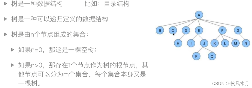
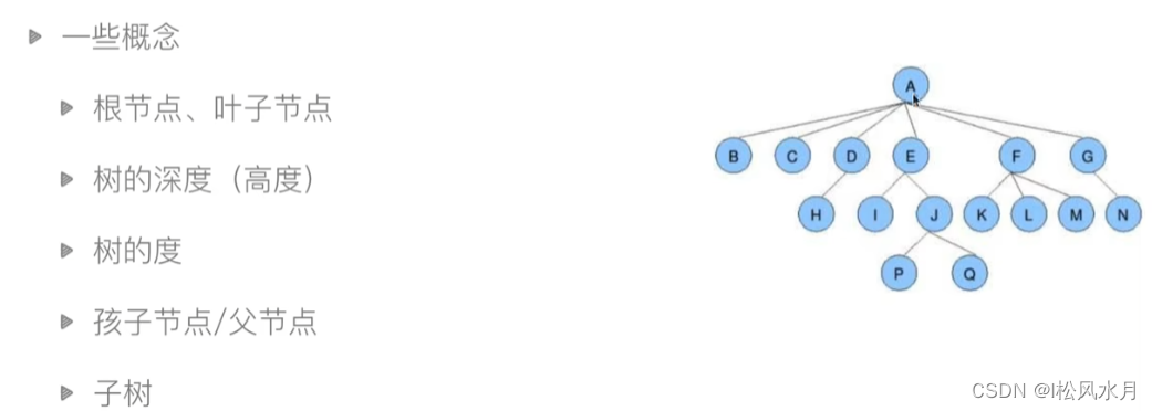
I briefly introduced the tree down when stacking the heap. A tree is a data structure. For example, a directory structure tree is a data structure that can be defined recursively. A tree is a collection of n nodes. If n=0, it is an empty tree; if n>0, it exists One node serves as the root node of the tree, and other nodes can be divided into m sets, each of which is itself a tree. Let's briefly demonstrate the operation of Linux files.
"""
模拟文件系统
"""


class Node:
    def __init__(self, name, type='dir'):
        self.name = name
        self.type = type
        self.children = []
        self.parent = None

    def __repr__(self):
        return self.name


class FileSystemTree:
    def __init__(self):
        self.root = Node("/")
        self.now = self.root

    def mkdir(self, name):
        # name要以 / 结尾
        if name[-1] != "/":
            name += "/"
        node = Node(name)
        # 连接子目录
        self.now.children.append(node)
        # 连接上级目录
        node.parent = self.now

    def ls(self):
        return self.now.children

    def cd(self, name):
        # 相对路径
        if name[-1] != "/":
            name += "/"
        if name == "../":
            self.now = self.now.parent
            return
        # 判断要进来的目录在不在
        for child in self.now.children:
            if child.name == name:
                self.now = child
                return
        raise ValueError("invlaid dir")


tree = FileSystemTree()
tree.mkdir("var/")
tree.mkdir("bin/")
tree.mkdir("usr/")

tree.cd("bin/")
tree.mkdir("python/")
print(tree.ls())
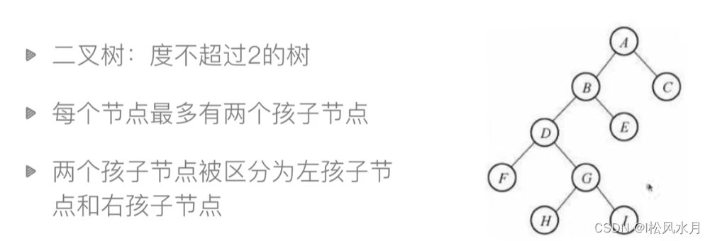
2.6.1. Binary tree
A node can be divided into at most two branches. Simply implement the following binary tree:

class BiTreeNode:
    def __init__(self, data):
        self.data = data
        self.lchild = None
        self.rchild = None

a = BiTreeNode("A")
b = BiTreeNode("B")
c = BiTreeNode("C")
d = BiTreeNode("D")
e = BiTreeNode("E")
f = BiTreeNode("F")
g = BiTreeNode("G")

e.rchild = g
e.lchild = a
a.rchild = c
g.rchild = f
c.rchild = d
c.lchild = b
root = e
print(root.lchild.rchild.data)
Binary tree traversal:
four ways, pre-order traversal, in-order traversal, post-order traversal, level traversal. The structure of the tree can be deduced based on the traversal results.
from collections import deque
class BiTreeNode:
    def __init__(self, data):
        self.data = data
        self.lchild = None
        self.rchild = None


a = BiTreeNode("A")
b = BiTreeNode("B")
c = BiTreeNode("C")
d = BiTreeNode("D")
e = BiTreeNode("E")
f = BiTreeNode("F")
g = BiTreeNode("G")

e.rchild = g
e.lchild = a
a.rchild = c
g.rchild = f
c.rchild = d
c.lchild = b

root = e


# 前序遍历
def pre_order(root):
    if root:
        print(root.data, end=",")
        pre_order(root.lchild)
        pre_order(root.rchild)


# 中序遍历
def in_order(root):
    if root:
        in_order(root.lchild)
        print(root.data, end=",")
        in_order(root.rchild)


# 后序遍历
def post_order(root):
    if root:
        in_order(root.lchild)
        in_order(root.rchild)
        print(root.data, end=",")


# 层次遍历
def layer_order(root):
    queue = deque()
    queue.append(root)
    # 只要队不空就一直访问
    while len(queue) > 0:
        node = queue.popleft()
        # 访问刚才出队的元素
        print(node.data, end=",")
        if node.lchild:
            queue.append(node.lchild)
        if node.rchild:
            queue.append(node.rchild)


pre_order(root)
print("\n")
in_order(root)
print("\n")
post_order(root)
print("\n")
layer_order(root)
You should be familiar with the pre-order traversal, in-order traversal and post-order traversal above, and be able to deduce the structure of the tree based on the given traversal results. Generally, two traversal results will be given for you to deduce.
2.6.2. Binary Search Tree
Second, the search tree is a binary tree and satisfies the property: Let x be a node of the binary tree. If y is a node in the left subtree of x, then y.key ≤ x.key;if y is a node in the right subtree of x, then y.key > x.key.
Operations of binary search tree: query, insert, delete
The implementation of insertion and query, take the following tree as an example:

class BiTreeNode:
    def __init__(self, data):
        self.data = data
        self.lchild = None  # 左孩子
        self.rchild = None  # 右孩子
        self.parent = None


class BST:
    def __init__(self, li=None):
        self.root = None
        if li:
            for val in li:
                self.insert_no_rec(val)

    # 递归方法
    def insert(self, node, val):
        if not node:
            node = BiTreeNode(val)
        elif val < node.data:
            node.lchild = self.insert(node.lchild, val)
            node.lchild.parent = node
        elif val > node.data:
            node.rchild = self.insert(node.rchild, val)
            node.rchild.parent = node
        return node

    # 普通方法
    def insert_no_rec(self, val):
        p = self.root
        # 空树,特殊处理
        if not p:
            self.root = BiTreeNode(val)
            return  # 空树
        while True:
            if val < p.data:
                if p.lchild:
                    p = p.lchild  # 左孩子不存在
                else:
                    p.lchild = BiTreeNode(val)
                    p.lchild.parent = p
                    return
            elif val > p.data:
                if p.rchild:
                    p = p.rchild
                else:
                    p.rchild = BiTreeNode(val)
                    p.rchild.parent = p
                    return
            else:
                return

    # 递归查询
    def query(self, node, val):
        if not node:
            return None
        if node.data < val:
            return self.query(node.rchild, val)
        elif node.data > val:
            return self.query(node.lchild, val)
        else:
            return

    # 非递归查询
    def query_no_rec(self, val):
        p = self.root
        while p:
            if p.data < val:
                p = p.lchild
            elif p.data > val:
                p = p.lchild
            else:
                return p
        return None

    # 前序遍历
    def pre_order(self, root):
        if root:
            print(root.data, end=",")
            self.pre_order(root.lchild)
            self.pre_order(root.rchild)

    # 中序遍历
    def in_order(self, root):
        if root:
            self.in_order(root.lchild)
            print(root.data, end=",")
            self.in_order(root.rchild)

    # 后序遍历
    def post_order(self, root):
        if root:
            self.in_order(root.lchild)
            self.in_order(root.rchild)
            print(root.data, end=",")


tree = BST([4, 5, 3, 7, 8, 1, 2, 9])
tree.pre_order(tree.root)
print("")
# 一定是升序序列
tree.in_order(tree.root)
print("")
tree.post_order(tree.root)
print("")
print(tree.query_no_rec(4).data)
Deletion:
When deleting, you need to pay attention to the following three situations:
-
If the node to be deleted is a leaf node, delete it directly

-
If the node to be deleted has only one child: connect this node's parent with the child, then delete the node.

-
If the node to be deleted has two children: delete the smallest node of its right subtree (the node has at most one right child) and replace the current node.

class BiTreeNode:
    def __init__(self, data):
        self.data = data
        self.lchild = None  # 左孩子
        self.rchild = None  # 右孩子
        self.parent = None


class BST:
    def __init__(self, li=None):
        self.root = None
        if li:
            for val in li:
                self.insert_no_rec(val)

    # 递归方法
    def insert(self, node, val):
        if not node:
            node = BiTreeNode(val)
        elif val < node.data:
            node.lchild = self.insert(node.lchild, val)
            node.lchild.parent = node
        elif val > node.data:
            node.rchild = self.insert(node.rchild, val)
            node.rchild.parent = node
        return node

    # 普通方法
    def insert_no_rec(self, val):
        p = self.root
        # 空树,特殊处理
        if not p:
            self.root = BiTreeNode(val)
            return  # 空树
        while True:
            if val < p.data:
                if p.lchild:
                    p = p.lchild  # 左孩子不存在
                else:
                    p.lchild = BiTreeNode(val)
                    p.lchild.parent = p
                    return
            elif val > p.data:
                if p.rchild:
                    p = p.rchild
                else:
                    p.rchild = BiTreeNode(val)
                    p.rchild.parent = p
                    return
            else:
                return

    # 递归查询
    def query(self, node, val):
        if not node:
            return None
        if node.data < val:
            return self.query(node.rchild, val)
        elif node.data > val:
            return self.query(node.lchild, val)
        else:
            return

    # 非递归查询
    def query_no_rec(self, val):
        p = self.root
        while p:
            if p.data < val:
                p = p.rchild
            elif p.data > val:
                p = p.lchild
            else:
                return p
        return None

    # 情况一:node是叶子结点,直接删掉
    def __remove_mode_1(self, node):
        # 先判断是不是根节点
        if not node.parent:
            self.root = None
        # 将子节点与父节点断绝联系
        if node == node.parent.lchild:
            node.parent.lchild = None
        else:
            node.parent.rchild = None

    # 情况2.1:要删除的节点node只有一个左孩子
    def __remove_node_21(self, node):
        # 先判断要删除的是不是根节点
        if not node.parent:
            # 如果要删除的是根节点,就把做孩子设置为根节点
            self.root = node.lchild
            # 子节点设置为父节点,父节点置为空
            node.lchild.parent = None
        # 判断这个删除的节点是父节点的左孩子还是右孩子
        elif node == node.parent.lchild:
            node.parent.lchild = node.lchild
            node.lchild.parent = node.parent
        else:
            node.parent.rchild = node.lchild
            node.lchild.parent = node.parent

    # 情况2.2:要删除的节点node只有一个右孩子(原理同上)
    def __remove_node_22(self, node):
        if not node.parent:
            self.root = node.rchild
        elif node == node.parent.lchild:
            node.parent.lchild = node.rchild
            node.rchild.parent = node.parent
        else:
            node.parent.rchild = node.rchild
            node.rchild.parent = node.parent

    # 要删除的节点既有左孩子,又有右孩子
    def delete(self, val):
        if self.root:  # 不是空树
            # 找到要删除的节点
            node = self.query_no_rec(val)
            # 判断节点是否存在
            if not node:
                return False
            # 判断节点的子节点情况
            if not node.lchild and not node.rchild:  # 叶子结点
                self.__remove_mode_1(node)
            elif not node.rchild:  # 2.1只有一个左孩子,这里的写法要注意,不能判断是否有右孩子,不然无法判断左孩子是否存在
                self.__remove_node_21(node)
            elif not node.lchild:  # 2.1只有一个右孩子
                self.__remove_node_22(node)
            else:  # 3.两个孩子都有
                min_node = node.rchild
                # 找到右子树最小的节点
                while min_node.lchild:
                    min_node = min_node.lchild
                node.data = min_node.data
                # 删除min_node
                if min_node.rchild:
                    self.__remove_node_22(min_node)
                else:
                    self.__remove_mode_1(min_node)

    # 前序遍历
    def pre_order(self, root):
        if root:
            print(root.data, end=",")
            self.pre_order(root.lchild)
            self.pre_order(root.rchild)

    # 中序遍历
    def in_order(self, root):
        if root:
            self.in_order(root.lchild)
            print(root.data, end=",")
            self.in_order(root.rchild)

    # 后序遍历
    def post_order(self, root):
        if root:
            self.in_order(root.lchild)
            self.in_order(root.rchild)
            print(root.data, end=",")


tree = BST([4, 5, 3, 7, 8, 1, 2, 9])
# 一定是升序序列
tree.in_order(tree.root)
print("")
tree.delete(4)
tree.in_order(tree.root)
print("")
output:
1,2,3,4,5,7,8,9,
1,2,3,5,7,8,9,
2.6.3. AVL tree
The time complexity of a binary tree is O ( longn ) O(longn)O ( l o n g n ) , but in the worst case, the binary tree is very skewed and branches to one side, as shown in the figure below. Thus leads to the AVL tree.

AVL tree: AVL tree is aSelf-balancing(The height difference between the trees on any two sides will not exceed 1) binary search tree.
AVL trees have the following properties:
- The absolute value of the difference between the heights of the left and right subtrees of the root cannot exceed 1
- The left and right subtrees of the root are balanced binary trees

As shown in the figure above, the balance factor is the height of the tree on the left minus the height of the tree on the right, and the absolute value will not exceed 1.
Since the AVL tree is required to be balanced, how do we insert data, and how to ensure that it is balanced when inserting? Let's look at the animation below.

From the animation above, we can see that if there is an imbalance during insertion, it can be turned into a balanced tree by rotation.
- Inserting a node may break the balance of the AVL tree, which can be corrected by rotation operation
- After inserting a node, only the balance of nodes on the path from the inserted node to the root node may be changed (colored path in animation). We need to find the first node that violates the equilibrium condition, call it
K.KThe difference in height between the two subtrees is 2.
There may be 4 situations in which the imbalance occurs:
-
Left-handed: the imbalance is due to the insertion into the right subtree of the right child of K

-
Right-handed: the imbalance is due to the insertion into the left subtree of the left child of K

-
Right-handed first - then left-handed: the imbalance is due to the insertion of the left subtree of the right child of K

-
Left-handed first - then right-handed: the imbalance is due to the insertion of the left and right subtrees of the left child of K

Memory method:
Right and left, left and right, right and left, left and right. Rotation is to exchange the superior-subordinate relationship.
The following shows an animation of four rotations:

AVL tree insertion rules, which stipulate that the right side of the balance factor is subtracted from the left side. If the inserted element is on the right side of the node, the node balance factor +1, if it comes from the left side, the node balance factor -1, and if there is a certain node in the middle. The absolute value of the balance factor If it is greater than 2, the node is rotated (four rotations are for four cases).
Code example:
# 导入之前创建好的类
from btree import BST, BiTreeNode


# 通过继承创建节点
class AVLNode(BiTreeNode):
    def __init__(self, data):
        BiTreeNode.__init__(self, data)
        # 节点平衡因子
        self.bf = 0


# 通过继承创建树
class AVLTree(BST):
    def __init__(self, li=None):
        BST.__init__(self, li)

    # 针对插入导致不平衡的旋转,不适用于删除情况
    def rotate_left(self, p, c):
        # 参照示例图写出下面的代码,进行旋转(节点交换)
        s2 = c.lchild
        p.rchild = s2
        # 判断s2是否是空的,不是空的再连接到父类,如果为None就不用连了
        if s2:
            s2.parent = p

        c.lchild = p
        p.parent = c
        # 更新bc
        p.bf = 0
        c.bf = 0
        # 返回最后的根节点
        return c

    # 针对插入导致不平衡的旋转,不适用于删除情况
    def rotate_right(self, p, c):
        s2 = c.rchild
        p.lchild = s2
        # 判断s2是否是空的
        if s2:
            s2.parent = p

        c.rchild = p
        p.parent = c
        # 更新bc
        p.bf = 0
        c.bf = 0
        # 返回最后的根节点
        return c

    def rotate_right_lef(self, p, c):
        # 通过给的示例图可以看到只有s2,s3的归属发生的变化
        g = c.lchild

        # 先右旋
        s3 = g.rchild
        c.lchild = s3
        if s3:
            s3.parent = c
        g.rchild = c
        # 这里不需要判断c是否为None,c不可能为None
        c.parent = g

        # 在左旋
        s2 = g.lchild
        p.rchild = s2
        if s2:
            s2.parent = g
        g.lchild = p
        p.parent = g

        # 更新bf
        if g.bf > 0:
            p.bf = -1
            c.bf = 0
        elif g.bf < 0:
            p.bf = 0
            c.bf = 1
        # s1~s4节点都没有,插入的是G节点
        else:
            p.bf = 0
            c.bf = 0

        # 返回最后的根节点
        return g

    def rotate_left_right(self, p, c):
        # 通过给的示例图可以看到只有s2,s3的归属发生的变化
        g = c.rchild

        # 先右旋
        s2 = g.lchild
        c.rchild = s2
        if s2:
            s2.parent = c
        g.lchild = c
        # 这里不需要判断c是否为None,c不可能为None
        c.parent = g

        # 在左旋
        s3 = g.rchild
        p.lchild = s3
        if s3:
            s3.parent = g
        g.rchild = p
        p.parent = g

        # 更新bf
        if g.bf > 0:
            p.bf = 0
            c.bf = -1
        elif g.bf < 0:
            p.bf = 1
            c.bf = 0
        # s1~s4节点都没有,插入的是G节点
        else:
            p.bf = 0
            c.bf = 0

        # 返回最后的根节点
        return g

    # 插入
    def insert_no_rec(self, val):
        # 1.插入:和二叉搜索树插入差不多
        p = self.root
        # 空树,特殊处理
        if not p:
            self.root = BiTreeNode(val)
            return  # 空树
        while True:
            if val < p.data:
                if p.lchild:
                    p = p.lchild  # 左孩子不存在
                else:
                    p.lchild = BiTreeNode(val)
                    p.lchild.parent = p
                    # node存储插入的节点
                    node = p.lchild
                    break
            elif val > p.data:
                if p.rchild:
                    p = p.rchild
                else:
                    p.rchild = BiTreeNode(val)
                    p.rchild.parent = p
                    node = p.rchild
                    break
            # 等于的时候什么也不做,不让节点有重复
            else:
                return

        # 更新平衡因子,从node的父节点开始,要保证父节点部位空
        while node.parent:
            # 1. 传递是从左子树来的,左子树更沉
            if node.parent.lchild == node:
                # 更新node.parent的bf -= 1
                if node.parent.bf < 0:  # 原来的node.parent =-1 ,更新之后变为-2
                    # 继续看node的哪边沉
                    g = node.parent.parent  # 保存节点的父节点的父节点,用于更新node,重新连接,目的就是为了连接旋转之后的子树
                    # 旋转前的子树的根
                    x = node.parent
                    if node.bf > 0:
                        n = self.rotate_left_right(node.parent, node)
                    else:
                        n = self.rotate_right(node.parent)
                    # 记得把n和g连接起来
                elif node.parent.bf > 0:  # 原来node.parent.bf = 1,更新之后变为0
                    # 变为0之后不需要再旋转了
                    node.parent.bf = 0
                    break
                else:
                    node.parent.bf = -1
                    node = node.parent
                    continue

                pass
            # 2. 传递是从右子树来的,右子树更沉
            else:
                # 更新node.parent的bf -= 1
                if node.parent.bf > 0:  # 原来的node.parent =1 ,更新之后变为2
                    # 继续看node的哪边沉
                    g = node.parent.parent
                    # 旋转前的子树的根
                    x = node.parent
                    if node.bf < 0:
                        n = self.rotate_right_lef(node.parent, node)
                    else:
                        n = self.rotate_left(node.parent, node)
                #         记得连起来
                elif node.parent.bf < 0:  # 原来的node.parent =-1 ,更新之后变为0
                    node.parent = 0
                    break
                else:  # 原来的node.parent =0 ,更新之后变为1
                    node.parent.bf = 1
                    node = node.ap
                    continue
            # 连接旋转后的子树
            n.parent = g
            # g不是空
            if g:
                if x == g.lchild:
                    g.lchild = n
                else:
                    g.rchild = n
                break
                pass
            else:
                self.root = n
                break


tree = AVLTree([9, 8, 7, 6, 5, 4, 3, 2, 1])
tree.pre_order(tree.root)
tree.in_order()
B-Tree of AVL tree extension: a node connects data, divided into three ways, small, medium and large, as shown in the following figure:

3. High-level examples of algorithms
In the previous blog post, we recorded the basic knowledge of data structures and algorithms. In this blog post, we will look at the advanced algorithms.
3.1. Greedy algorithm
Greedy algorithm (also known as greedy algorithm) means that when solving a problem, always make the best choice at present. That is to say, without considering the overall optimality, what he made is a local optimal solution in a certain sense.
The greedy algorithm does not guarantee that the optimal solution will be obtained, but the solution of the greedy algorithm is the optimal solution on some problems. It is necessary to judge whether a problem can be calculated by a greedy algorithm.
Look at a classic question:
suppose the store owner needs to change n yuan. The denominations of coins are: 100 yuan, 50 yuan, 20 yuan, 5 yuan, and 1 yuan. How to make change so that the number of coins required is the least?
t = [100, 50, 20, 5, 1]


def change(t, n):
    m = [0 for _ in range(len(t))]
    for i, money in enumerate(t):
        m[i] = n // money
        n = n % money
    return m, n


print(change(t, 376))
output:
([3, 1, 1, 1, 1], 0)
Let's look at another backpack problem:
a thief finds n items in a certain store, and the i-th item is worth v yuan and weighs w; kg. He hopes to take as much value as possible, but his backpack can only hold up to W kilograms. Which goods should he take away?
There are two cases:
- 0-1 Backpack: For a commodity, the thief either takes it whole or keeps it. It is not possible to take only part of an item, or to take an item multiple times. (The product is gold bars)
- Score Backpack: (The commodity is gold sand) Score Backpack: For a commodity, the thief can take any part of it. (calculate unit weight)
Let's first look at how to write the score backpack (see behind the 0-1 backpack):
def fractional_backpack(goods, w):
    m = [0 for _ in range(len(goods))]
    total_value = 0
    for i, (price, weight) in enumerate(goods):
        # 判断能不能一次拿完
        if w >= weight:
            m[i] = 1
            w -= weight
            total_value += price
        # 只取一部分
        else:
            m[i] = w / weight
            W = 0
            total_value += m[i] * price
    return total_value, m


print(fractional_backpack(goods, 50))
(240.0, [1, 1, 0.6666666666666666])
Looking at a problem of concatenating the largest number:
there are n non-negative integers, which are concatenated into an integer in the way of string concatenation. How to concatenate to make the largest integer?
Example: 32,94,128,1286,6,71 The largest integer that can be concatenated and divided is 94716321286128
Idea: compare the first digit, compare the size of the end when the first digit is the same (splice the front and back into a string to compare the size).
from functools import cmp_to_key

li = [32, 94, 128, 1286, 6, 71]


def xy_cmp(x, y):
    if x + y < y + x:
        return 1
    elif x + y > y + x:
        return -1
    else:
        return 0


def number_join(li):
    li = list(map(str, li))
    li.sort(key=cmp_to_key(xy_cmp))
    return "".join(li)


print(number_join(li))
output:
94716321286128
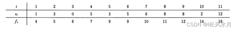
Looking at a classic problem: the activity selection problem
- Assuming that there are n activities, these activities will occupy the same space, and the space can only be used by one activity at a time.
- Each activity has a start time si s_isiand end time fi f_ifi(The time in the title is expressed as an integer), indicating that the activity is in [ si s_isi, f i f_i fi) interval occupies the space.
- Q: Which events can be scheduled to maximize the number of events held at the venue?
Ideas:
- Greedy conclusion: The activity that ends first must be part of the optimal solution.
- Proof: Assume that a is the activity that ends first among all activities, and b is the activity that ends first in the optimal solution.
- If a=b, the conclusion holds.
- If a ≠ ba \ne ba=b , then the end time of b must be later than the end time of a, then replace b in the optimal solution with a at this time, and a must not overlap with other activity times in the optimal solution, so the replaced solution is also the optimal solution
activities = [(1, 4), (3, 5), (0, 6), (5, 8), (3, 9), (6, 10), (8, 11), (8, 12), (2, 14), (12, 16)]
activities.sort(key=lambda x: x[1])


def activity_selection(a):
    # 排序好的第一个肯定是最优的
    res = [a[0]]
    for i in range(1, len(a)):
        if a[i][0] >= res[-1][1]:
            res.append(a[i])
    return res


print(activity_selection(activities))
output:
[(1, 4), (5, 8), (8, 11), (12, 16)]
Summary: The greedy algorithm is actually an optimization problem, and it also has limitations, leading to the following dynamic programming algorithm.
3.2. Dynamic programming
Dynamic Programming (Dynamic Programming) is an algorithm design technique for solving complex problems. It is mainly used for optimization problems, that is, to find the optimal solution (maximum or minimum) under the given constraints. The core idea of dynamic programming is to decompose a complex problem into a series of sub-problems, and use the solutions of the sub-problems to construct the solution of the original problem.
Let's look directly at the question, let's first look at a very common Fibonacci number: F=Fn-1+Fn-2.
Use recursive and non-recursive methods to solve the nth term of the Fibonacci sequence
"""
递归函数
子问题重复计算,当计算的项数非常大的时候会非常慢,时间换空间
"""
import time


def fibancci(n):
    if n == 1 or n == 2:
        return 1
    else:
        return fibancci(n - 2) + fibancci(n - 1)


start = time.time()
print(fibancci(30))
end = time.time()
print(end - start)
'''
非递归函数,空间换时间
'''


def fibancci_no_recurision(n):
    f = [0, 1, 1]
    for i in range(n - 2):
        num = f[-1] + f[-2]
        f.append(num)
    return f[n]


start = time.time()
print(fibancci_no_recurision(30))
end = time.time()
print(end - start)
output:
832040
0.16655564308166504
832040
0.0
It can be seen that the non-recursive time is close to 0s, and the recursive time is much longer than the non-recursive time. The non-recursive solution method can embody the idea of dynamic programming (DP).
Dynamic programming idea = optimal substructure (recursive) + repeated word problem (save the required sub-problem)
Let's look at another steel bar cutting problem:
a company sells steel bars, and the relationship between the selling price and the length of the steel bars is as follows
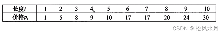
Question: Given a steel bar with a length of n and the above price list, find a plan for cutting the steel bar to maximize the total profit.
Take a look at the optimal solution method:
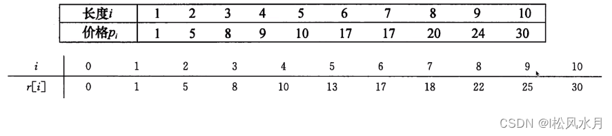
From the table above, we can see that the optimal solution of the length of the last m plane can be added through the previous optimal solution, which is somewhat similar to the Fibonacci sequence.
Idea:
Let the optimal profit value after cutting the steel bar with length n be rn r_nrn, can get the recursive formula rn = max ( P n , r 1 + rn − 1 , r 2 + rn − 2 , ⋅ ⋅ , rn − 1 + r 1 ) r_n=max(P_n,r_1 +r_{n- 1},r_2 +r_{n-2},··,r_{n-1}+r_1)rn=max(Pn,r1+rn−1,r2+rn−2,⋅⋅,rn−1+r1) the first parameterpn p_npnIndicates no cutting, and the other n-1 parameters represent another n-1 different cutting schemes. For scheme i=1,2,...,n-1, the steel bar is cut into two sections of length i and ni. As the sum of the optimal benefits of cutting two segments, examine all i, and choose the plan with the largest profit.
Core: When a small optimal solution can build a large optimal solution, dynamic programming ideas can be used.
The above idea can also be changed, one side is cut and the other side is not cut:
cut a section of length i from the left side of the steel bar, and only continue to cut the remaining section on the right side, and no longer cut the left side, recursive Simplified to rn = max ( pi + rn − i ) , i ∈ [ 1 , n ] r_n=max(p_i+r_{ni}), i \in [1,n]rn=max(pi+rn−i),i∈[1,n ]
The scheme without cutting can be described as: the length of the left section is n, the income is p_n, the length of the remaining section is 0, and the income is r_o=0.
def cut_rod_recurision_1(p, n):
    if n == 0:
        return 0
    else:
        res = p[n]
        for i in range(1, n):
            res = max(res, cut_rod_recurision_1(p, i) + cut_rod_recurision_1(p, n - i))
        return res


def cut_rod_recurision_2(p, n):
    if n == 0:
        return 0
    else:
        res = 0
        for i in range(1, n + 1):
            res = max(res, p[i] + cut_rod_recurision_2(p, n - i))
        return res


start = time.time()
print(cut_rod_recurision_1(p, 9))
end = time.time()
print(end - start)
start = time.time()
print(cut_rod_recurision_2(p, 9))
end = time.time()
print(end - start)
output:
25
0.0019943714141845703
25
0.0
The above two ways of writing are recursive calls, but the second way is obviously faster than the first way, but it is not good, it is time for space, very slow. Lead to the following dynamic programming, space for time, and save the intermediate calculation results.
def cut_rod_dp(p, n):
    r = [0]
    # 循环n次
    for i in range(1, n + 1):
        res = 0
        for j in range(1, i + 1):
            res = max(res, p[j] + r[i - j])
        r.append(res)
    return r[n]
Using dynamic programming can greatly reduce the time complexity. Bottom-up view, intermediate results saved.
The above is the maximum cost obtained, so how should we cut to get the maximum cost?
def cut_rod_extend(p, n):
    r = [0]
    s = [0]
    for i in range(1, n + 1):
        res_r = 0
        res_s = 0
        for j in range(1, i + 1):
            if p[j] + r[i - j] > res_r:
                res_r = p[j] + r[i - j]
                res_s = j
        r.append(res_r)
        s.append(res_s)
    return r[n], s


def cut_rod_solution(p, n):
    r, s = cut_rod_extend(p, n)
    ans = []
    while n > 0:
        ans.append(s[n])
        n -= s[n]
    return ans

print(cut_rod_solution(p, 9))
output:
[3, 6]
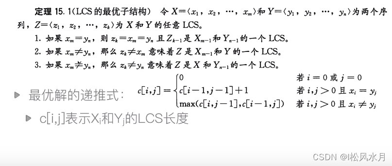
Looking at the problem of a longest common subsequence:
a subsequence of a sequence is a sequence obtained by deleting several elements in the sequence. Example: "ABCD" and "BDF" are both subsequences of "ABCDEFG".
Longest Common Subsequence (LCS) Problem: Given two sequences X and Y, find the common subsequence with the largest length of X and Y.
Example: X="ABBCBDE" Y="DBBCDB"LCS(XY)="BBCD
application scenario: string similarity comparison, gene sequence comparison
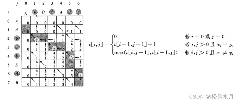
def lcs_length(x, y):
    m = len(x)
    n = len(y)
    c = [[0 for _ in range(n + 1)] for _ in range(m + 1)]
    for i in range(1, m + 1):
        for j in range(1, n + 1):
            if x[i - 1] == y[j - 1]:
                c[i][j] = c[i - 1][j - 1] + 1
            else:
                c[i][j] = max(c[i - 1][j], c[i][j - 1])
    for _ in c:
        print(_)
    return c[m][n]


print(lcs_length("ABCBDAB", "BDCABA"))
output:
[0, 0, 0, 0, 0, 0, 0]
[0, 0, 0, 0, 1, 1, 1]
[0, 1, 1, 1, 1, 2, 2]
[0, 1, 1, 2, 2, 2, 2]
[0, 1, 1, 2, 2, 3, 3]
[0, 1, 2, 2, 2, 3, 3]
[0, 1, 2, 2, 3, 3, 4]
[0, 1, 2, 2, 3, 4, 4]
4
The cutting length is given above, how to cut it? That is, the circled letters in the figure above correspond to the oblique arrows.
def lcs(x, y):
    m = len(x)
    n = len(y)
    c = [[0 for _ in range(n + 1)] for _ in range(m + 1)]
    b = [["-" for _ in range(n + 1)] for _ in range(m + 1)]  # ↖表示左上方,↑表示上方,←表示左方
    for i in range(1, m + 1):
        for j in range(1, n + 1):
            if x[i - 1] == y[j - 1]:  # i,j位置上的字符匹配的时候,来自于左上方
                c[i][j] = c[i - 1][j - 1] + 1
                b[i][j] = "↖"  # 将箭头方向改为"↖"
            elif c[i - 1][j] >= c[i][j - 1]:  # 将大于号改为大于等于号
                c[i][j] = c[i - 1][j]
                b[i][j] = "↑"
            else:
                c[i][j] = c[i][j - 1]
                b[i][j] = "←"  # 将箭头方向改为"←"
    return c, b


def lcs_trackback(x, y):
    c, b = lcs(x, y)
    i = len(x)
    j = len(y)
    res = []
    while i > 0 and j > 0:
        if b[i][j] == "↖":
            res.append(x[i - 1])
            i -= 1
            j -= 1
        elif b[i][j] == "↑":
            i -= 1
        else:
            j -= 1
    return "".join(reversed(res))


c, b = lcs("ABCBDAB", "BDCABA")
for _ in b:
    print(_)
res = lcs_trackback("ABCBDAB", "BDCABA")
print(res)
output:
['-', '-', '-', '-', '-', '-', '-']
['-', '↑', '↑', '↑', '↖', '←', '↖']
['-', '↖', '←', '←', '↑', '↖', '←']
['-', '↑', '↑', '↖', '←', '↑', '↑']
['-', '↖', '↑', '↑', '↑', '↖', '←']
['-', '↑', '↖', '↑', '↑', '↑', '↑']
['-', '↑', '↑', '↑', '↖', '↑', '↖']
['-', '↖', '↑', '↑', '↑', '↖', '↑']
BCBA
Looking at a Euclidean algorithm to find the greatest common divisor:
Euclidean algorithm: gcd(a, b)= gcd(b,a mod b) Example: gcd(60,21)= gcd(21, 18) = gd(18,3)= gcd(3,0
) = 3
# 递归
def gcd1(a, b):
    if b == 0:
        return a
    else:
        return gcd1(b, a % b)


# 非递归
def gcd2(a, b):
    while b > 0:
        r = a % b
        a = b
        b = r
    return a


print(gcd1(12, 4))
print(gcd2(12, 4))
output:
4
4