After a month of experience, this timing anomaly detection tool is too silky

1 Introduction to adtk

The data of intelligent operation and maintenance AIOps is basically in the form of time series , and anomaly detection alarms are an important part of AIOps. The author recently used the adtk python library when processing time series data, and I will share it with you here.

What is adtk?

adtk (Anomaly Detection Toolkit) is a python toolkit for unsupervised anomaly detection , which provides common algorithms and processing functions:

Simple and effective anomaly detection algorithm ( detector **)**
Unusual feature processing ( transformers )
Process flow control ( Pipe )

2 installation

pip install adtk

3. adtk data requirements

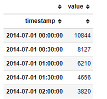
Time series data mainly includes time and corresponding indicators (such as cpu, memory, quantity, etc.). Data analysis in python is generally a pandas DataFrame, and adtk requires that the index of the input data must be DatetimeIndex.

pandas provides methods for time generation and processing of time series.

pd.date_range

stamps = pd.date_range("2012-10-08 18:15:05", periods=4, freq="D")
# DatetimeIndex(['2012-10-08 18:15:05', '2012-10-09 18:15:05',
#           '2012-10-10 18:15:05', '2012-10-11 18:15:05'],
#          dtype='datetime64[ns]', freq='D')

pd.Timestamp

tmp = pd.Timestamp("2018-01-05") + pd.Timedelta("1 day")
print(tmp, tmp.timestamp(), tmp.strftime('%Y-%m-%d'))
# 2018-01-06 00:00:00 1515196800.0 2018-01-06
pd.Timestamp( tmp.timestamp(), unit='s', tz='Asia/Shanghai')
# Timestamp('2018-01-06 08:00:00+0800', tz='Asia/Shanghai')

pd.to_datetime

adtk provides is validate_seriesto verify the validity of time series data, such as whether it is in chronological order

import pandas as pd
from adtk.data import validate_series
from adtk.visualization import plot
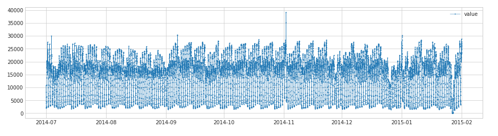
df = pd.read_csv('./data/nyc_taxi.csv', index_col="timestamp", parse_dates=True)
df = validate_series(df)
plot(df)

Technology Exchange

Technology must learn to share and communicate, and it is not recommended to work behind closed doors. One person can go fast, and a group of people can go farther.

Good articles are inseparable from the sharing and recommendation of fans, dry data, data sharing, data, and technical exchange improvement, all of which can be obtained by adding the communication group. The group has more than 200 friends. The best way to add notes is: source + interest directions, making it easy to find like-minded friends.

Method ①, Add WeChat account: dkl88194, Remarks: from CSDN + technical communication
Method ②, WeChat search official account: Python learning and data mining, background reply: add group

4. Abnormal feature processing (transformers)

transformersMany time series feature processing methods are provided in adtk :

Generally, we obtain the characteristics of the time series, usually sliding according to the time window , and collect the statistical characteristics on the time window ;
There is also a decomposition of seasonal trends to distinguish which are seasonal parts and which are trend parts
Time series dimensionality reduction mapping: For fine-grained time series data, the amount of data is large, which is not efficient for detection algorithms. The dimensionality reduction method can preserve the main trend and other characteristics of the time series while reducing the dimensionality and providing time efficiency. This is particularly effective for time series classification using CNN. adtk mainly provides pca-based dimensionality reduction and reconstruction methods, which are mainly applied to multidimensional time series.

4.1 Sliding window

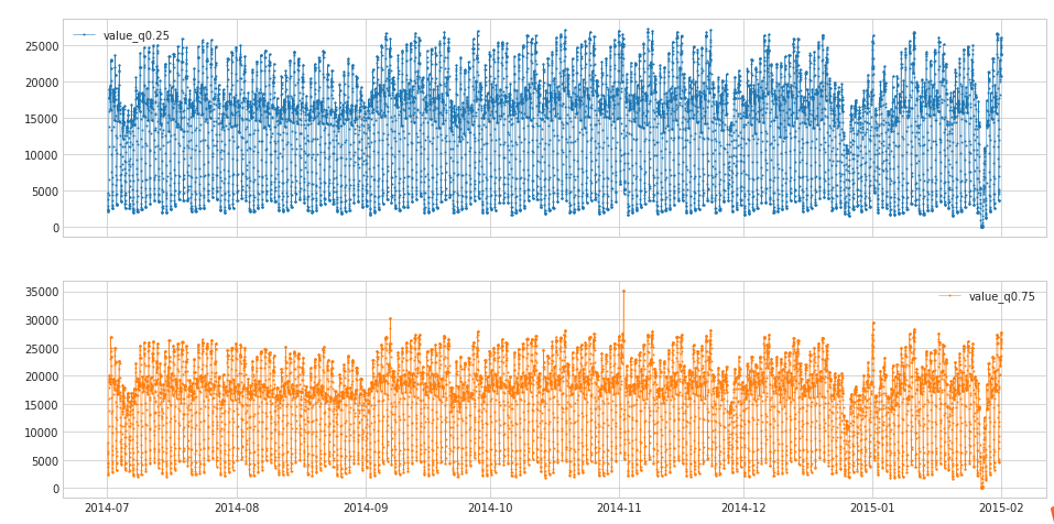
atdk offers single wide mouth RollingAggregateand 2 window DoubleRollingAggregatesliding ways. Statistical features support mean, median, summary, maximum, minimum, quantile, variance, standard deviation, skewness, kurtosis, histogram, etc., ['mean', 'median', 'sum', 'min', 'max', 'quantile', 'iqr', 'idr', 'count', 'nnz', 'nunique', 'std', 'var', 'skew', 'kurt', 'hist']where

' iqr ': is the difference between the quantile 75% and 25%
' idr ': is the quantile 90% and 10% interpolation
RollingAggregate

import pandas as pd
from adtk.data import validate_series
from adtk.transformer import RollingAggregate
from adtk.transformer import DoubleRollingAggregate
s = pd.read_csv('./data/nyc_taxi.csv', index_col="timestamp", parse_dates=True)
s = validate_series(s)

s_transformed = RollingAggregate(agg='quantile',agg_params={
    
    "q": [0.25, 0.75]}, window=5).transform(s)

DoubleRollingAggregate provides the difference of statistical features between two windows , such as the first 5 minutes and the last 5 minutes, the difference of the mean, etc. aggThe parameters are the same as those in RollingAggregate, and the newly added parameters diffmainly measure the function of the gap:

import pandas as pd
from adtk.data import validate_series
from adtk.transformer import DoubleRollingAggregate
s = pd.read_csv('./data/ec2_cpu_utilization_53ea38.csv', index_col="timestamp", parse_dates=True)
s = validate_series(s)

s_transformed = DoubleRollingAggregate(
    agg="median",
    window=5,
    diff="diff").transform(s)

parameter:

' diff ': back minus front
‘rel_diff’: Relative difference between values of aggregated metric (right minus left divided left). Only applicable if the aggregated metric is scalar.
' abs_rel_diff ': (back-front)/front, relative difference
' l1 ': l1 regular
' l2 ': l2 regular

4.2 Seasonal dismantling

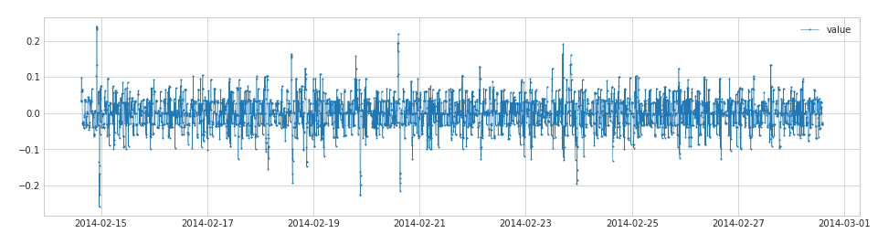
Time series can be disassembled into trend, seasonal and residual components. ClassicSeasonalDecompositionThese three parts are disassembled in atdk , and the trend and seasonal parts are removed, and the residual part is returned.

freq : set the seasonal period
trend : You can set whether to keep the trend

from adtk.transformer import ClassicSeasonalDecomposition
 
s = pd.read_csv('./data/nyc_taxi.csv', index_col="timestamp", parse_dates=True)
s = validate_series(s)
 
s_transformed = ClassicSeasonalDecomposition().fit_transform(s)

s_transformed = ClassicSeasonal
Decomposition(trend=True).fit_transform(s)

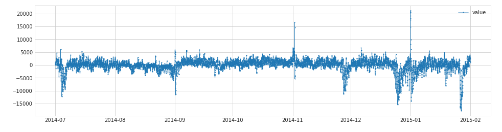
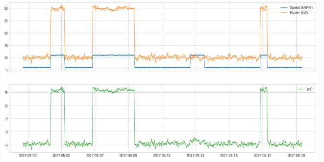
4.3 Dimensionality reduction and reconstruction

The pca provided by adtk performs dimensionality reduction to principal components PcaProjectionand reconstruction methods for data PcaReconstruction.

df = pd.read_csv('./data/generator.csv', index_col="Time", parse_dates=True)
df = validate_series(df)

from adtk.transformer import PcaProjection
s = PcaProjection(k=1).fit_transform(df)
plot(pd.concat([df, s], axis=1), ts_linewidth=1, ts_markersize=3, curve_group=[("Speed (kRPM)", "Power (kW)"), "pc0"]);

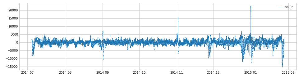
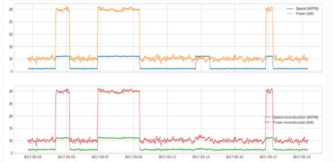
from adtk.transformer import PcaReconstruction
df_transformed = PcaReconstruction(k=1).fit_transform(df).rename(columns={
    
    
                "Speed (kRPM)": "Speed reconstruction (kRPM)",
                "Power (kW)": "Power reconstruction (kW)"})
plot(pd.concat([df, df_transformed], axis=1), ts_linewidth=1, ts_markersize=3,
     curve_group=[("Speed (kRPM)", "Power (kW)"),
                  ("Speed reconstruction (kRPM)", 
                   "Power reconstruction (kW)")]);

5. Anomaly detection algorithm (detector)

Adtk mainly provides unsupervised or rule- based time series detection algorithms, which can be used for conventional anomaly detection.

Detecting Outliers Outliers are data points that differ significantly from normal data. adtk mainly provides adtk.detector.ThresholdAD adtk.detector.QuantileAD adtk.detector.InterQuartileRangeAD adtk.detector.GeneralizedESDTestADthe detection algorithm included.

ThresholdAD

"""
adtk.detector.ThresholdAD(low=None, high=None)
参数：
low：下限，小于此值，视为异常
high：上限，大于此值，视为异常
原理：通过认为设定上下限来识别异常
总结：固定阈值算法
"""

from adtk.detector import ThresholdAD
threshold_ad = ThresholdAD(high=30, low=15)
anomalies = threshold_ad.detect(s)

QuantileAD

adtk.detector.QuantileAD(low=None, high=None)
参数：
low：分位下限，范围(0,1)，当low=0.25时，表示Q1
high：分位上限，范围(0,1)，当low=0.25时，表示Q3
原理：通过历史数据计算出给定low与high对应的分位值Q_low,Q_high，小于Q_low或大于Q_high，视为异常
总结：分位阈值算法

from adtk.detector import QuantileAD
quantile_ad = QuantileAD(high=0.99, low=0.01)
anomalies = quantile_ad.fit_detect(s)

InterQuartileRangeAD

adtk.detector.InterQuartileRangeAD(c=3.0)

**Parameters: **c: The coefficient of the quantile distance, used to determine the upper and lower limits, which can be float or (float,float)

Principle : When c is float, it is calculated through historical data Q3+c*IQRas the upper limit value, and it is considered abnormal if it is greater than the upper limit value. c=(float1,float2)At that time , it is calculated through historical data (Q1-c1*IQR, Q3+c2*IQR)as a normal range, and it is considered abnormal if it is not within the normal range

Summary : Boxplot Algorithm

from adtk.detector import InterQuartileRangeAD
iqr_ad = InterQuartileRangeAD(c=1.5)
anomalies = iqr_ad.fit_detect(s)

GeneralizedESDTestAD

adtk.detector.GeneralizedESDTestAD(alpha=0.05)

parameter:

alpha : Significance level, the smaller the alpha, the more likely the identified anomaly is a true anomaly.
Principle : After taking the difference between the value of the sample point and the mean value of the sample, divide it by the standard deviation of the sample, take the maximum value, calculate the threshold value through the t distribution, and compare the threshold value to determine the abnormal point.

A brief description of the calculation steps:

Set the significant level alpha, usually 0.05
Specify the outlier ratio h, if h=5%, it means that there are 2 outlier points in 50 samples
Calculate the mean mu and standard deviation sigma of the data set, take the difference between all samples and the mean, take the absolute value, and then divide by the standard deviation to find the maximum value and get esd_1
In the remaining sample points, repeat step 3 to get h esd values
Calculate critical value for each esd value: lambda_i (calculated using t distribution)
Count whether each esd is greater than lambda_i, if it is greater than that, you are considered abnormal

from adtk.detector import GeneralizedESDTestAD
esd_ad = GeneralizedESDTestAD(alpha=0.3)
anomalies = esd_ad.fit_detect(s)

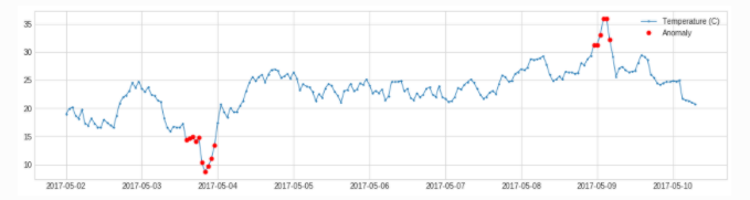
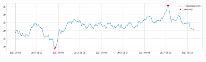
mutation :

The manifestation of Spike and Level Shift anomalies is not outliers, but through comparison with neighboring points , that is, sudden increase or sudden drop. adtk provides adtk.detector.PersistADand adtk.detector.LevelShiftADdetection methods

PersistAD

adtk.detector.PersistAD(window=1, c=3.0, side='both', min_periods=None, agg='median')

parameter:

window: reference window length, can be int, str
c: Quantile range multiple, used to determine the upper and lower limit range
side: detection range, when it is 'positive', it detects a sudden increase, when it is 'negative', it detects a sudden drop, when it is 'both', it detects both a sudden increase and a sudden drop
min_periods: The minimum number in the reference window, less than this number will report an exception, the default is None, which means that each time point must have a value
agg: the calculation method of statistics in the reference window, because the current value is compared with the statistics generated in the reference window, so the data in the reference window must be calculated as statistics, default
Accept 'median', which means the median value of the reference window

principle:

Use a sliding window to traverse the historical data, and make a difference between the one-bit data behind the window and the statistics in the reference window to obtain a new time series s1;
Calculate (Q1-c_IQR, Q3+c_IQR) of s1 as the normal range;
If the difference between the current value and the statistic in its reference window is not within the normal range in 2, it is considered abnormal.

Tuning parameters:

window: The larger the model, the less sensitive it is, and it is less likely to be disturbed by spikes
c: The larger the value, the larger the normal range for data with large fluctuations, and the smaller the normal range for data with less fluctuations
min_periods: The tolerance for missing values, the larger the value, the less it is allowed to have too many missing values
agg: The aggregation method of statistics, related to the characteristics of statistics, such as 'median' is not easily affected by extreme values
Summary: First calculate a new time series, and then use the boxplot for anomaly detection

  from adtk.detector import PersistAD
  persist_ad = PersistAD(c=3.0, side='positive')
  anomalies = persist_ad.fit_detect(s)

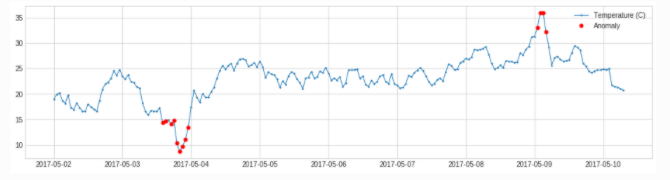
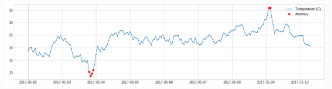
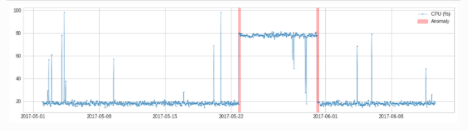
LevelShiftAD

adtk.detector.LevelShiftAD(window, c=6.0, side='both', min_periods=None)

parameter:

window: support (10,5), means to use two adjacent sliding windows, the median value in the left window represents the reference value, and the median value in the right window represents the current value
c: The larger the value, the larger the normal range for data with large fluctuations, and the smaller the normal range for data with less fluctuations, the default is 6.0
side: detection range, when it is 'positive', it detects a sudden increase, when it is 'negative', it detects a sudden drop, when it is 'both', it detects both a sudden increase and a sudden drop
min_periods: The minimum number in the reference window, less than this number will report an exception, the default is None, which means that each time point must have a value

principle:

This model is used to detect mutations. Compared with PersistAD, it has stronger anti-jitter ability and is less prone to false positives.

from adtk.detector import LevelShiftAD
level_shift_ad = LevelShiftAD(c=6.0, side='both', window=5)
anomalies = level_shift_ad.fit_detect(s)

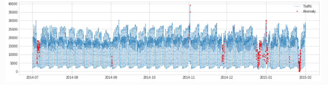
seasonal

adtk.detector.SeasonalAD

adtk.detector.SeasonalAD(freq=None, side='both', c=3.0, trend=False)

SeasonalAD is mainly processed and judged according to ClassicSeasonalDecomposition.

parameter:

freq: seasonal period
c: The larger the value, the larger the normal range for data with large fluctuations, and the smaller the normal range for data with less fluctuations, the default is 6.0
side: detection range, when it is 'positive', it detects a sudden increase, when it is 'negative', it detects a sudden drop, when it is 'both', it detects both a sudden increase and a sudden drop
trend: whether to consider the trend

from adtk.detector import SeasonalAD
seasonal_ad = SeasonalAD(c=3.0, side="both")
anomalies = seasonal_ad.fit_detect(s)
plot(s, anomaly=anomalies, ts_markersize=1, anomaly_color='red', 
     anomaly_tag="marker", anomaly_markersize=2);

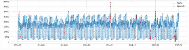
pipe combination algorithm

from adtk.pipe import Pipeline
steps = [
    ("deseasonal", ClassicSeasonalDecomposition()),
    ("quantile_ad", QuantileAD(high=0.995, low=0.005))
]
pipeline = Pipeline(steps)
anomalies = pipeline.fit_detect(s)
plot(s, anomaly=anomalies, ts_markersize=1, anomaly_markersize=2, 
     anomaly_tag="marker", anomaly_color='red');

6. Summary

This paper introduces ADTK, an unsupervised algorithmic toolkit for time series anomaly detection. ADTK provides simple anomaly detection algorithms and time series feature processing functions, I hope it will be helpful to you. Summarized as follows:

adtk requires the input data to be datetimeIndex tovalidate_series verify the validity of the data and make the time orderly
adtk single window and double window sliding, processing statistical features
adtk decomposes the seasonal part of the time series to obtain the residual part of the time series, which can be used to judge the abnormal point
adtk supports outlier, mutation, and seasonal anomaly detection. By fit_detectobtaining the abnormal point sequence, you can also Pipelineconnect multiple abnormal detection algorithms