semantic segmentation

Semantic Segmentation refers to the task of dividing an image into several regions and assigning semantic labels to each region. It is an important technology in computer vision and is widely used in areas such as autonomous driving, medical image analysis, and geographic information systems.

Different from traditional image segmentation tasks, semantic segmentation not only needs to divide the image into several regions, but also needs to assign semantic labels to each region. For example, in autonomous driving, semantic segmentation can segment areas such as roads, vehicles, and pedestrians, and assign corresponding semantic labels to each area to help vehicles drive autonomously. In medical image analysis, semantic segmentation can segment different tissue structures (such as organs, muscles, bones, etc.), and analyze and diagnose them.

The implementation methods of semantic segmentation can be mainly divided into region-based methods and pixel-based methods. Region-based methods segment an image into a series of regions, and then classify each region and assign a corresponding semantic label. Pixel-based methods directly classify each pixel and assign it a corresponding semantic label. At present, the method based on deep learning has become the mainstream method for semantic segmentation, among which the method based on convolutional neural network (CNN) is the most common. Commonly used semantic segmentation models include FCN, SegNet, U-Net, DeepLab, etc.

In the field of computer vision, there are two other important issues similar to semantic segmentation, namely image segmentation and instance segmentation. We briefly distinguish them from semantic segmentation here.
Image segmentation divides an image into several component regions, and methods for this type of problem usually exploit the correlation between pixels in the image. It does not require label information about image pixels during training, nor can it guarantee that the segmented regions have the semantics we want when predicting.
Instance segmentation is also called simultaneous detection and segmentation, which studies how to identify the pixel-level regions of each target instance in an image. Different from semantic segmentation, instance segmentation needs to distinguish not only semantics but also different target instances. For example, if there are two dogs in the image, instance segmentation needs to distinguish which of the two dogs the pixel belongs to.

data set

One of the most important datasets for semantic segmentation is Pascal VOC2012.

download dataset

%matplotlib inline
import os
import torch
import torchvision
from d2l import torch as d2l
#@save
d2l.DATA_HUB['voc2012'] = (d2l.DATA_URL + 'VOCtrainval_11-May-2012.tar',
                           '4e443f8a2eca6b1dac8a6c57641b67dd40621a49')

voc_dir = d2l.download_extract('voc2012', 'VOCdevkit/VOC2012')

read dataset

#@save
def read_voc_images(voc_dir, is_train=True):
    """读取所有VOC图像并标注"""
    txt_fname = os.path.join(voc_dir, 'ImageSets', 'Segmentation',
                             'train.txt' if is_train else 'val.txt')
    mode = torchvision.io.image.ImageReadMode.RGB
    with open(txt_fname, 'r') as f:
        images = f.read().split()
    features, labels = [], []
    for i, fname in enumerate(images):
        features.append(torchvision.io.read_image(os.path.join(
            voc_dir, 'JPEGImages', f'{
      
      fname}.jpg')))
        labels.append(torchvision.io.read_image(os.path.join(
            voc_dir, 'SegmentationClass' ,f'{
      
      fname}.png'), mode))
    return features, labels

train_features, train_labels = read_voc_images(voc_dir, True)

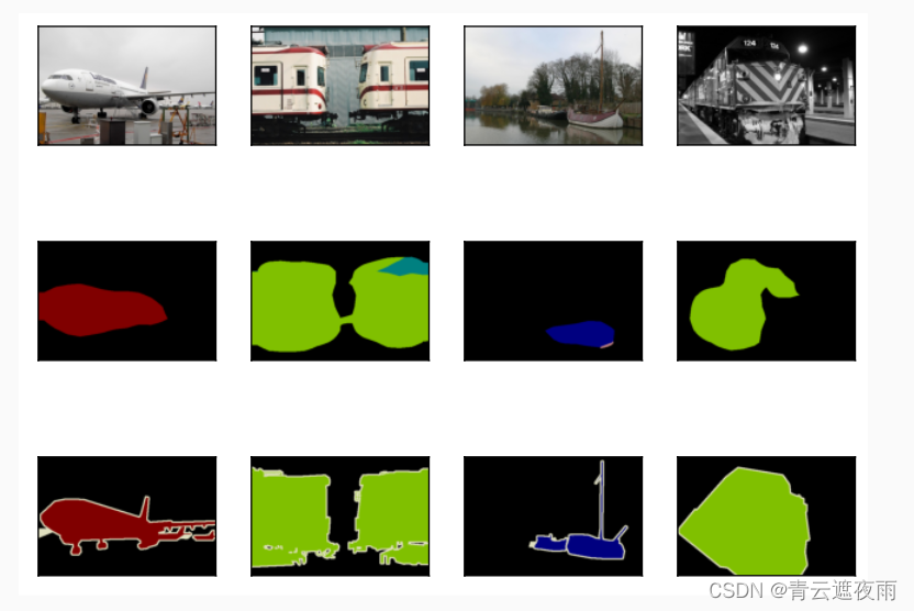
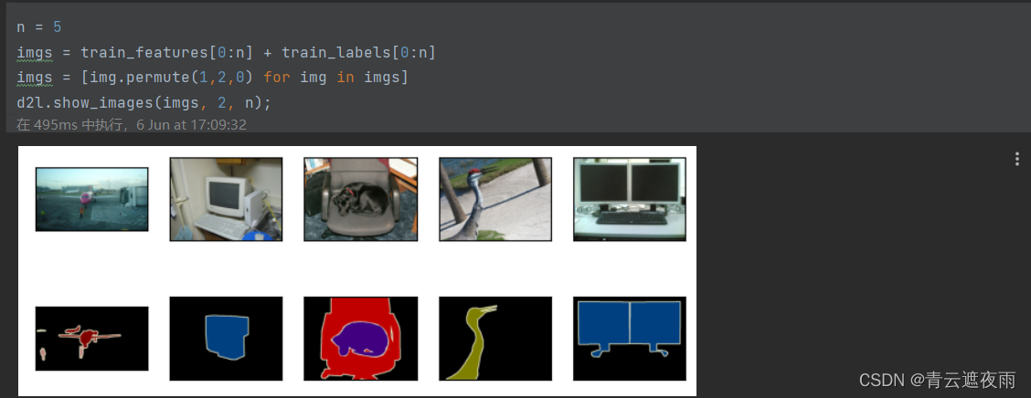
Below we plot the first 5 input images and their labels. In label images, white and black represent border and background, respectively, while other colors correspond to different categories.

n = 5
imgs = train_features[0:n] + train_labels[0:n]
imgs = [img.permute(1,2,0) for img in imgs]
d2l.show_images(imgs, 2, n);

insert image description here
Next, we enumerate RGB color values and class names.

VOC_COLORMAP = [[0, 0, 0], [128, 0, 0], [0, 128, 0], [128, 128, 0],
                [0, 0, 128], [128, 0, 128], [0, 128, 128], [128, 128, 128],
                [64, 0, 0], [192, 0, 0], [64, 128, 0], [192, 128, 0],
                [64, 0, 128], [192, 0, 128], [64, 128, 128], [192, 128, 128],
                [0, 64, 0], [128, 64, 0], [0, 192, 0], [128, 192, 0],
                [0, 64, 128]]

#@save
VOC_CLASSES = ['background', 'aeroplane', 'bicycle', 'bird', 'boat',
               'bottle', 'bus', 'car', 'cat', 'chair', 'cow',
               'diningtable', 'dog', 'horse', 'motorbike', 'person',
               'potted plant', 'sheep', 'sofa', 'train', 'tv/monitor']

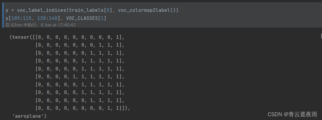
With the two constants defined above, we can conveniently look up the class index of each pixel in the label. We define the voc_colormap2label function to construct a mapping from the above RGB color values to category indices, and the voc_label_indices function to map RGB values to category indices in the Pascal VOC2012 dataset.

#@save
def voc_colormap2label():
    """构建从RGB到VOC类别索引的映射"""
    colormap2label = torch.zeros(256 ** 3, dtype=torch.long)
    for i, colormap in enumerate(VOC_COLORMAP):
        colormap2label[
            (colormap[0] * 256 + colormap[1]) * 256 + colormap[2]] = i
    return colormap2label

Specifically, the code uses a method of converting RGB color values into a unique integer, that is, the values of the three channels of R, G, and B are multiplied by 25 6 2 256^ $25 6^{2}$ 、 $256^1$ 、 $256^0$ , and add them together. This converts a triplet of RGB color values into a unique integer.

#@save
def voc_label_indices(colormap, colormap2label):
    """将VOC标签中的RGB值映射到它们的类别索引"""
    colormap = colormap.permute(1, 2, 0).numpy().astype('int32')
    idx = ((colormap[:, :, 0] * 256 + colormap[:, :, 1]) * 256
           + colormap[:, :, 2])
    return colormap2label[idx]

Specifically, the function first converts the RGB values in the "colormap" tensor to an integer tensor "idx" of size (H, W). This is by multiplying the values of the three channels R, G, and B by $256^2$ 、 $256^1$ 、 $256^0$ , and then add them together. This integer is then used as an index to extract the corresponding class index from the "colormap2label" tensor. These category indices form a new tensor "idx" of the same shape as the "colormap" tensor, where each element corresponds to a pixel in the "colormap" tensor.

insert image description here

Preprocess data

In semantic segmentation, doing so requires remapping the predicted pixel classes back to the original size of the input image. Such a mapping may not be precise enough, especially in different semantically segmented regions. To avoid this problem, we crop the image to a fixed size instead of rescaling. Specifically, we crop the same region of the input image and label using random cropping in image augmentation.

#@save
def voc_rand_crop(feature, label, height, width):
    """随机裁剪特征和标签图像"""
    rect = torchvision.transforms.RandomCrop.get_params(
        feature, (height, width))
    feature = torchvision.transforms.functional.crop(feature, *rect)
    label = torchvision.transforms.functional.crop(label, *rect)
    return feature, label

imgs = []
for _ in range(n):
    imgs += voc_rand_crop(train_features[0], train_labels[0], 200, 300)

imgs = [img.permute(1, 2, 0) for img in imgs]
d2l.show_images(imgs[::2] + imgs[1::2], 2, n);

The function uses torchvision.transforms.RandomCrop.get_params() to get a random crop rectangle, and then uses the torchvision.transforms.functional.crop() function to crop the input feature image and label image. Finally, the function returns the cropped feature image and label image. Specifically, the function achieves random cropping through the following steps:

Use torchvision.transforms.RandomCrop.get_params() to get a random cropping rectangle with height and width respectively.
Use torchvision.transforms.functional.crop() to crop the input feature image and label image, and the cropped rectangle is the random rectangle obtained in the previous step.
Return the cropped feature image and label image.

Custom Semantic Segmentation Dataset Class

#@save
class VOCSegDataset(torch.utils.data.Dataset):
    """一个用于加载VOC数据集的自定义数据集"""

    def __init__(self, is_train, crop_size, voc_dir):
        self.transform = torchvision.transforms.Normalize(
            mean=[0.485, 0.456, 0.406], std=[0.229, 0.224, 0.225])
        self.crop_size = crop_size
        features, labels = read_voc_images(voc_dir, is_train=is_train)
        self.features = [self.normalize_image(feature)
                         for feature in self.filter(features)]
        self.labels = self.filter(labels)
        self.colormap2label = voc_colormap2label()
        print('read ' + str(len(self.features)) + ' examples')

    def normalize_image(self, img):
        return self.transform(img.float() / 255)

    def filter(self, imgs):
        return [img for img in imgs if (
            img.shape[1] >= self.crop_size[0] and
            img.shape[2] >= self.crop_size[1])]

    def __getitem__(self, idx):
        feature, label = voc_rand_crop(self.features[idx], self.labels[idx],
                                       *self.crop_size)
        return (feature, voc_label_indices(label, self.colormap2label))

    def __len__(self):
        return len(self.features)

This is a custom dataset class VOCSegDataset for loading Pascal VOC datasets. The dataset class provides the following methods:

init (self, is_train, crop_size, voc_dir): constructor, used to initialize the dataset. The function accepts three parameters:

is_train: A boolean indicating whether this dataset is for training or testing.
crop_size: A tuple indicating the size of the random cropped image.
voc_dir: Data set storage path.

normalize_image(self, img): Used to normalize the image.

filter(self, imgs): Used to filter out images whose size is smaller than crop_size.

getitem (self, idx): Used to get an item in the dataset. This function accepts an index parameter idx and returns a tuple (feature, label), where feature represents the feature image and label represents the corresponding label image.

len (self): Used to get the number of samples in the dataset.

In the constructor, the dataset class first uses the read_voc_images() function to read the images and labels in the dataset, and uses the filter() method to filter out images whose size is smaller than crop_size. Then, the dataset class uses the normalize_image() method to normalize each feature image, and uses the voc_rand_crop() and voc_label_indices() methods to achieve random cropping and label mapping of feature images and label images. Finally, the dataset class returns the cropped feature and label images in the getitem () method.

The main function of this dataset class is to convert the Pascal VOC dataset into the Dataset type in PyTorch, so that the DataLoader class provided by PyTorch can be used to batch process the data when training the model.

crop_size = (320, 480)
voc_train = VOCSegDataset(True, crop_size, voc_dir)
voc_test = VOCSegDataset(False, crop_size, voc_dir)

batch_size = 64
train_iter = torch.utils.data.DataLoader(voc_train, batch_size, shuffle=True,
                                    drop_last=True,
                                    num_workers=d2l.get_dataloader_workers())
for X, Y in train_iter:
    print(X.shape)
    print(Y.shape)
    break

Integrate all components

#@save
def load_data_voc(batch_size, crop_size):
    """加载VOC语义分割数据集"""
    voc_dir = d2l.download_extract('voc2012', os.path.join(
        'VOCdevkit', 'VOC2012'))
    num_workers = d2l.get_dataloader_workers()
    train_iter = torch.utils.data.DataLoader(
        VOCSegDataset(True, crop_size, voc_dir), batch_size,
        shuffle=True, drop_last=True, num_workers=num_workers)
    test_iter = torch.utils.data.DataLoader(
        VOCSegDataset(False, crop_size, voc_dir), batch_size,
        drop_last=True, num_workers=num_workers)
    return train_iter, test_iter

Fully Convolutional Network

The fully convolutional model is a special convolutional neural network that can classify or segment an input image at the pixel level and output a segmentation result with the same size as the input image. A fully convolutional model usually consists of a convolutional layer, a deconvolutional layer, and a pooling layer, where the convolutional layer is used to extract image features, the deconvolutional layer is used to restore the feature image to the original image size, and the pooling layer is used to Reduce the size of feature images.

Fully convolutional models are most commonly used for image segmentation tasks such as semantic segmentation, instance segmentation, and edge detection, among others. Among them, the semantic segmentation task is to assign each pixel in the image to its corresponding category, while the instance segmentation task is to assign each object instance in the image to a different category.

A classic structure of the fully convolutional model is U-Net, which consists of two parts: an encoder and a decoder. Encoders usually employ a combination of convolutional and pooling layers to extract image features and reduce the size of feature images. The decoder uses deconvolution layers and skip connections to restore the feature image to the original image size, and fuses the feature image in the encoder with the feature image in the decoder.

When training a fully convolutional model, the cross-entropy loss function is usually used to measure the difference between the model output and the true label, and the backpropagation algorithm is used to update the model parameters. Since the output of a fully convolutional model is a segmented image, it usually needs to be flattened into a vector when computing the loss function.

construction model

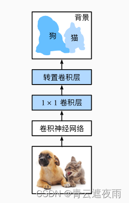
Let's take a look at the most basic design of a fully convolutional network model. As shown in the figure below, the full convolutional network first uses the convolutional neural network to extract image features, and then passes $1\times 1$ The convolutional layer transforms the number of channels into the number of categories, and finally transforms the height and width of the feature map into the size of the input image through the transposed convolutional layer. Therefore, the model output has the same height and width as the input image, and the final output channel contains the class prediction for the pixel at that spatial location.
insert image description here
Below, we use the ResNet-18 model pretrained on the ImageNet dataset to extract image features, and denote this network as pretrained_net. The last few layers of the ResNet-18 model include global average pooling layers and fully connected layers, whereas they are not required in fully convolutional networks.
insert image description here
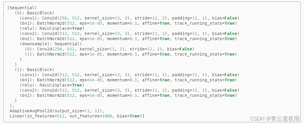
Next, we create a fully convolutional network net. It replicates most of the pre-training layers in ResNet-18, except for the global average pooling layer at the end and the fully connected layer closest to the output.

net = nn.Sequential(*list(pretrained_net.children())[:-2])

Given an input with a height of 320 and a width of 480, the forward propagation of net reduces the height and width of the input to the original $\frac{1}{32}$ , immediately 10 and 15.

X = torch.rand(size=(1, 3, 320, 480))
net(X).shape

insert image description here
Next use $1\times 1$ convolutional layer converts the number of output channels to the number of classes (21 classes) of the Pascal VOC2012 dataset. Finally, we need to increase the height and width of the feature map by a factor of 32, thus changing it back to the height and width of the input image. Since $(320 - 64 + 16 * 2 + 32) /32 = 10$ and $(480 - 64 + 16 * 2 + 32) /32 = 15$ , we construct a stride of $32$ transposed convolution layer, and set the height and width of the convolution kernel to $64$ , filled with $16$ . We can see that if the stride is $s$ , filled with $s /2$ (assuming $s$ is an integer) and the height and width of the convolution kernel are $2 s$ , the transposed convolution kernel will amplify the input height and width by $s$ times.

Initialize the transposed convolution layer

In image processing, we sometimes need to enlarge the image, that is, upsampling. Bilinear interpolation is one of the commonly used upsampling methods, and it is also often used to initialize transposed convolutional layers.

Upsampling is a method of increasing a low resolution image or signal to a high resolution. Bilinear interpolation is one of the commonly used upsampling methods, which can generate higher-resolution images by interpolating existing low-resolution images.

In bilinear interpolation, it is assumed that a low-resolution image is to be sampled twice, that is, each pixel becomes a $\times 2$ pixel blocks. For pixels in each new pixel block, bilinear interpolation is calculated from the surrounding four known pixel value values. Specifically, for a new pixel ( x , y ) in the target image $(x, y)$ , its gray value can be calculated by the following steps:

Find target pixel $(x, y)$ $(x_1, y_1)$ in the original low-resolution image $(x_{1}, y_{1})$ ， $x_2, y_1)$ ， $x_1, y_2)$ ， $x_2, y_2)$ , in which $x_1, y_1)$ 和 $x_2, y_2)$ is the closest to $(x, y)$ , $x_1, y_2)$ 和 $x_2, y_1)$ are the other two pixels.

Calculate target pixel $(x, y)$ and the distance between four known pixels, namely $d_{1} = \sqrt{(x-x_1)^2 + (y -y_1)^2}$ ， $d_{2} = \sqrt{(x-x_2)^2 + (y-y_1)^2}$ ， $d_{3} = \sqrt{(x-x_1)^2 + (y-y_2)^2}$ ， $d_{4} = \sqrt{(x-x_2)^2 + (y-y_2)^2}$ 。

Calculate target pixel $(x, y)$ , the gray value of the surrounding four pixels is used for weighted average, and the weight is inversely proportional to the distance between the target pixel and the four known pixels. Right now:

$\frac{1}{d_{1}d_{3}}f(x_1, y_1) + \frac{1}{d_{2}d_{3}}f(x_2, y_1) + \frac{1}{d_{1}d_{4}}f(x_1, y_2) + \frac{1}{d_{2}d_{4}}f(x_2, y_2)$

where $f(x_1, y_1)$ ， $f(x_2, y_1)$ ， $f(x_1, y_2)$ ， $f(x_2, y_2)$ respectively represent the gray values of four known pixels.

With bilinear interpolation, we can upsample a low-resolution image to a higher resolution, resulting in a sharper image.

def bilinear_kernel(in_channels, out_channels, kernel_size):
    factor = (kernel_size + 1) // 2
    if kernel_size % 2 == 1:
        center = factor - 1
    else:
        center = factor - 0.5
    og = (torch.arange(kernel_size).reshape(-1, 1),
          torch.arange(kernel_size).reshape(1, -1))
    filt = (1 - torch.abs(og[0] - center) / factor) * \
           (1 - torch.abs(og[1] - center) / factor)
    weight = torch.zeros((in_channels, out_channels,
                          kernel_size, kernel_size))
    weight[range(in_channels), range(out_channels), :, :] = filt
    return weight

This is a function for generating a bilinear interpolation convolution kernel. Its input includes the number of input channels, the number of output channels, and the size of the convolution kernel, and its output is a tensor of shape (in_channels, out_channels, kernel_size, kernel_size) representing the bilinear interpolation convolution kernel generated by this function .

Specifically, the function first calculates the position of the center of the convolution kernel, and then generates a tensor filt of shape (kernel_size, kernel_size), where each element of filt represents the weight of the corresponding position in the bilinear interpolation convolution kernel . Finally, the function generates a tensor weight of shape (in_channels, out_channels, kernel_size, kernel_size) according to the number of input channels and output channels, where each element of weight represents the weight of the corresponding position in the bilinear interpolation convolution kernel. Specifically, weight[i, j, :, :] represents the bilinear interpolation kernel from the i-th input channel to the j-th output channel.

This function can be used to define a bilinear interpolation convolutional layer in a convolutional neural network, which upsamples the input tensor to a higher resolution.

Fully convolutional networks initialize transposed convolutional layers with upsampling with bilinear interpolation. For $1\times 1$ convolutional layer, we use Xavier initialization parameters.

W = bilinear_kernel(num_classes, num_classes, 64)
net.transpose_conv.weight.data.copy_(W);

train

def loss(inputs, targets):
    return F.cross_entropy(inputs, targets, reduction='none').mean(1).mean(1)

num_epochs, lr, wd, devices = 5, 0.001, 1e-3, d2l.try_all_gpus()
trainer = torch.optim.SGD(net.parameters(), lr=lr, weight_decay=wd)
d2l.train_ch13(net, train_iter, test_iter, loss, trainer, num_epochs, devices)

predict

When predicting, we need to normalize the input image in each channel and convert it into the four-dimensional input format required by the convolutional neural network.

def predict(img):
    X = test_iter.dataset.normalize_image(img).unsqueeze(0)
    pred = net(X.to(devices[0])).argmax(dim=1)
    return pred.reshape(pred.shape[1], pred.shape[2])

To visualize the predicted class for each pixel, we map the predicted classes back to their labeled colors in the dataset.

def label2image(pred):
    colormap = torch.tensor(VOC_COLORMAP, device=devices[0])
    X = pred.long()
    return colormap[X, :]

The images in the test dataset vary in size and shape. Since the model uses a transposed convolution layer with a stride of 32, when the height or width of the input image cannot be divisible by 32, the height or width of the output of the transposed convolution layer will deviate from the size of the input image. In order to solve this problem, we can intercept multiple rectangular areas in the image whose height and width are integer multiples of 32, and perform forward propagation on the pixels in these areas respectively. Note that the union of these regions needs to completely cover the input image. When a pixel is covered by multiple regions, the average value of the output of the transposed convolutional layer in the forward propagation of different regions can be used as the input of the softmax operation to predict the category.

For simplicity, we only read a few larger test images, and start from the upper left corner of the image to intercept the shape of $320\times 480$ is used for prediction. For these test images, we print their intercepted regions one by one, then print the prediction results, and finally print the labeled categories.