Saturation forecast
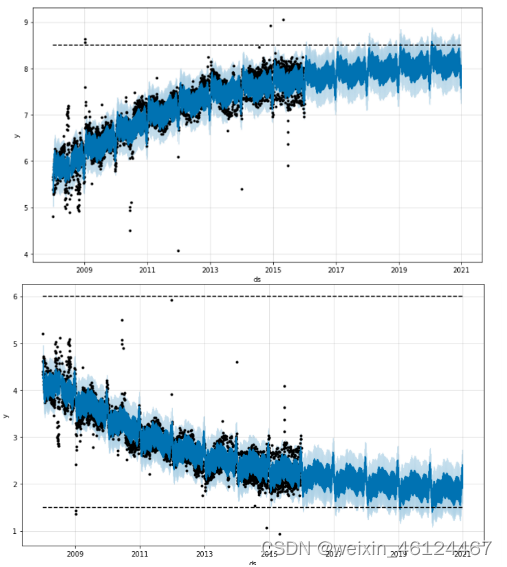
By default, Prophet uses a linear model for forecasting. When forecasting growth, there are usually some maximum attainable points: total market size, total population size, etc. This is called carrying capacity, and the forecast should saturate at this point.
Saturation forecast
What does predicting when it will reach saturation
mean?
Under a certain resource condition, the growth curve of the number of rabbits shows a trend like a sigmoid function, and we are predicting that trend.
That environmental resource can make the maximum number of rabbits exist as the cap set below
The trend of the curve changes like a sigmoid function
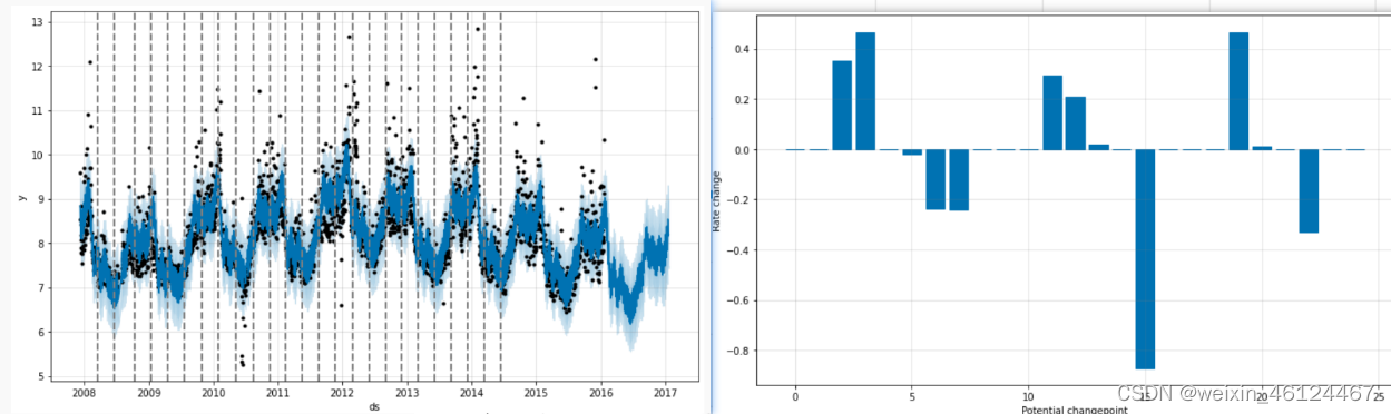
trend change point
By default, Prophet will automatically detect these change points and allow the trend to adjust appropriately. However, if you wish to have finer control over this process (e.g. the Prophet missed a rate change, or overfitted the rate change in the history), then you can use several input parameters.
My understanding is that the curve of the number of inflection points relative to the magnitude of the inflection point is shown on the right
Comparison of seasonality, holiday effects and regressors
: holiday effects are generally calculated on an annual basis, and seasonality is more subdivided into time periods
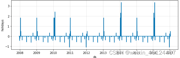
holiday
What does the holiday effect mean?
Based on the time of the specified holiday or national statutory holiday (usually based on the year) as a key point, it will be given priority when building the model
If you have holidays or other recurring events to model, you must create a data frame for them. It has two columns (holiday and ds) and a row for each occurrence of a holiday. It must include all events of the holiday, both past (in terms of historical data) and future (in terms of making predictions). If they do not repeat in the future, Prophet will model them and then not include them in the forecast.
My understanding:
holidays will be used as a factor affecting the change of the curve, and we will analyze the time period of holidays separately
Two ways:
specify the date and time for analysis (naming this time period is similar to supplementing holidays)
use python's built-in legal holidays of various countries, no need to define the time period yourself
The result of this operation is that there is an additional column of analysis data, which is the holiday
Add holidays:
custom holiday
code
m = Prophet(holidays=holidays)
m.fit(df)
national legal holidays
m = Prophet(holidays=holidays)
m.add_country_holidays(country_name='US')
m.fit(df)
Adjust how well the curve fits for holidays, and
if you find that holidays are overfitting, you can smooth them by adjusting their prior scale with the parameter holidays_prior_scale . By default, this parameter defaults to 10, which provides very little regularization. Reducing this parameter suppresses the holiday effect:
Code:
m = Prophet(holidays=holidays, holidays_prior_scale=0.05).fit(df)
forecast = m.predict(future)
forecast[(forecast['playoff'] + forecast['superbowl' ]).abs() > 0][
['ds', 'playoff', 'superbowl']][-10:]
seasonal
Seasonal Fourier order
What's the meaning?
Based on the data in recent years, establish a periodic model through periodicity (yearly, weekly, daily), and use Fourier series to fit the curve
Seasonality is estimated using partial Fourier sums. See the paper for full details, and this figure on Wikipedia to illustrate how partial Fourier sums can approximate arbitrary periodic signals. The number of terms in the partial sum (order) is a parameter that determines the rate of seasonality. To illustrate this, consider the Peyton Manning data from the quickstart. The default Fourier order for annual seasonality is 10, which produces the following fit:
Principle:
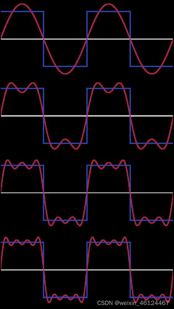
The default Fourier order is 10
from prophet.plot import plot_yearly
m = Prophet().fit(df)
a = plot_yearly(m)
Modify the Fourier order, the higher the order, the better the fitting accuracy
Note
The default values are usually suitable, but they can be increased when the seasonality needs to adapt to higher frequency changes, and is usually less smooth. When instantiating the model, the Fourier order can be specified for each built-in seasonality, here increased to 20:
from prophet.plot import plot_yearly
m = Prophet(yearly_seasonality=20).fit(df)
a = plot_yearly(m)
What is the difference between ??? and the smooth adjustment of the seasonal curve below? ? ? ?
Specify custom seasonality
The default seasonality (yearly, weekly, daily), if you want to add monthly seasonality, you need to add it manually
What does it mean here?
Use the Prophet model to calculate the weekly seasonal closure, and add a custom seasonal calculation at the same time, using every 30.5 days as a cycle to calculate the periodicity of the month. Summarize
all the data according to a 30.5-day cycle to summarize the relationship curve of a month's cycle change
代码
m = Prophet(weekly_seasonality=False)
m.add_seasonality(name=‘monthly’, period=30.5, fourier_order=5)
To adjust for this specified seasonality, adjust the fit of the seasonality
Note:
If you find that holidays are overfitting, you can smooth them by adjusting their prior scale with the parameter holidays_prior_scale . By default, this parameter is 10, which provides very little regularization. Reducing this parameter suppresses the holiday effect:
m = Prophet()
m.add_seasonality(
name=‘weekly’, period=7, fourier_order=3, prior_scale=0.1)
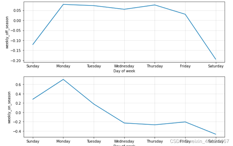
What does seasonality dependent on other factors
mean?
The data set originally had very little sales between February and August. For example, the approach below the yearly graph above is similar to this idea: Divide the data set into two data sets from February to August and January, September, October, November, and December The set calculates the periodicity of the two "quarters" separately! ! !
Here is an example: divide the peak season and off-season time period in a year, and do periodic analysis
def is_nfl_season(ds):
date = pd.to_datetime(ds)
return (date.month > 8 or date.month < 2)
df[‘on_season’] = df[‘ds’].apply(is_nfl_season)
df[‘off_season’] = ~df[‘ds’].apply(is_nfl_season)
m = Prophet(weekly_seasonality=False)
m.add_seasonality(name=‘weekly_on_season’, period=7, fourier_order=3, condition_name=‘on_season’)
m.add_seasonality(name=‘weekly_off_season’, period=7, fourier_order=3, condition_name=‘off_season’)
future[‘on_season’] = future[‘ds’].apply(is_nfl_season)
future[‘off_season’] = ~future[‘ds’].apply(is_nfl_season)
forecast = m.fit(df).predict(future)
fig = m.plot_components(forecast)
extra regressor
I don't know what this is