SalsaNext: Fast, Uncertainty-Aware Semantic Segmentation of LiDAR Point Clouds for Autonomous Driving
0. Summary
This paper presents a complete real-time 3D LiDAR point cloud for Uncertain Semantic Segmentation by SalsaNext. SalsaNext is the next version of SalsaNet [1], the encoder unit of the encoder-decoder architecture has a set of ResNet blocks and the residual block of the decoder part combined with upsampled features. Compared to SalsaNet, we introduce a new context module, replace the ResNet encoder module with a new atrous residual convolution with gradually increasing receptive field of view and add pixel shuffling layers in the decoder . Furthermore, we also switch from strided convolution to average pooling and apply a central dropout strategy. To directly optimize the Jaccard index, we further combine the weighted cross-entropy loss with the value-list ´asz-Softmax loss [2]. We ended up adding Bayesian to compute the epistemic and aleatoric uncertainties for each point cloud. We provide a comprehensive quantitative evaluation on the Semantic-KITTI dataset [3], which shows that SalsaNext outperforms other semantic segmentation networks ranked first in the Semantic-KITTI leaderboard. We also release the source code https://github.com/TiagoCortinhal/SalsaNext.
1 Introduction
Scene understanding is a necessary prerequisite for self-driving cars. Semantic segmentation helps gain a rich understanding of the scene by predicting meaningful class labels for each individual sensory data point. Achieving such fine-grained semantic predictions in real-time accelerates fully autonomous driving to a large extent.
However, safety-critical systems, such as self-driving cars, require not only highly accurate but also reliable predictions with a consistent measure of uncertainty. This is because quantitative uncertainty measurements can be propagated to subsequent units, such as decision modules, to lead to safe maneuver planning or emergency braking, which is extremely important in safety-critical systems. Therefore, combining semantic segmentation predictions with robust confidence estimates can greatly strengthen the notion of safe autonomy.
Advanced deep neural networks have recently made great leaps in generating accurate and reliable semantic segmentation with real-time performance. However, most of these methods rely on camera images [4], [5], while relatively few contributions discuss semantic segmentation of 3D LiDAR data [6], [7]. The main reason is that, unlike camera images, which provide dense measurements in a grid-like structure, LiDAR point clouds are relatively sparse, unstructured, and have uneven sampling, although LiDAR scanners have wider fields of view and return more accurate distance measurement.
As comprehensively described in [8], there exist two mainstream deep learning approaches that only address semantic segmentation of 3D LiDAR data: pointwise and projection-based neural networks (see Figure 1). The former directly operates on raw 3D points without any preprocessing steps, while the latter projects point clouds into various formats, such as 2D image views or high-dimensional volumetric representations. As shown in Figure 1, there is a clear separation between the two approaches in terms of accuracy, runtime, and memory consumption. For example, projection-based methods (shown as green circles in Figure 1) achieve state-of-the-art accuracy while running significantly faster. While point networks (red squares) have slightly fewer parameters, they cannot scale efficiently to large point sets due to limited processing power and thus require longer runtimes. It is also important to note that both pointwise and projection-based methods in the literature lack an uncertainty measure, i.e. a confidence score.
In this work, we introduce a novel neural network architecture that performs uncertainty-aware semantic segmentation of full 3D lidar point clouds in real-time. Our proposed network is built on the SalsaNet model [1], hence the name SalsaNext. The SalsaNet model has an encoder-decoder skeleton, where the encoder unit consists of a series of ResNet blocks, and the decoder part upsamples and fuses the features extracted in the residual blocks. In SalsaNext proposed here, our contributions lie in the following aspects:
- To capture global contextual information in full 360◦ LiDAR scans, we introduce a new contextual module before the encoder, which consists of a stack of residual dilated convolutions that fuse receptive fields at various scales.
- To increase the receptive field, we replace the ResNet block in the encoder with a new combination of a set of dilated convolutions (rate 2), where each convolution has a different kernel size (3, 5, 7). We further concatenate the convolutional outputs and combine with residual connections to produce branch-like structures.
- To avoid any checkerboard effect during upsampling, we replace the transposed convolutional layer in the SalsaNet decoder with a pixel shuffling layer [9], which directly utilizes feature maps to upsample the input with less computation.
- In order to enhance the role of very basic features (such as edges and curves) in the segmentation process, the dropout process is changed by omitting the first and last network layers in the dropout process.
- To have a lighter model, average pooling is employed instead of strided convolutions in the encoder.
- To improve segmentation accuracy by optimizing the average cross-joint score (i.e. Jaccard index), the weighted cross-entropy loss in SalsaNet is combined with the Lov'asz-Softmax loss [2].
- To further estimate the epistemic (model) and arbitrary (observational) uncertainties for each 3D LiDAR point, the deterministic SalsaNet model was converted to a stochastic format by applying a Bayesian process.
All these contributions form the SalsaNext model presented here, a probabilistic derivation of SalsaNet with significantly better segmentation performance. The input to SalsaNext is a rasterized image of a full LiDAR scan, where each image channel stores position, depth, and intensity cues in a panoramic view format. The final network output is a pointwise classification score along with an uncertainty measure.
To the best of our knowledge, this is the first work that shows both epistemic and aleatoric uncertainty estimation for the LiDAR point cloud segmentation task. Computing both types of uncertainty is critical in safe autonomous driving, as epistemic uncertainty can indicate the limits of segmentation models, while arbitrary uncertainty highlights the noise of sensor observations used for segmentation.
Quantitative and qualitative experiments on the SemanticKITTI dataset [3] show that the proposed SalsaNext significantly outperforms other state-of-the-art networks in terms of pixel segmentation accuracy while having fewer parameters and thus requiring less computation time. SalsaNext is #1 on the Semantic-KITTI leaderboard.
Note that we also release our source code and trained models to encourage further research on the topic.
2. Related work
In this section, recent work on semantic segmentation of 3D point cloud data is summarized. Then, there will be a brief review of the literature related to uncertainty estimation in Bayesian neural networks.
A. Semantic Segmentation of 3D Point Clouds
Recently, great progress has been made in semantic segmentation of 3D LiDAR point clouds using deep neural networks [1], [6], [7], [10], [11]. The core difference between these advanced methods lies not only in the network design, but also in the representation of point cloud data.
Fully convolutional network [12], encoder-decoder structure [13] and multi-branch model [5] etc. are mainstream network architectures for semantic segmentation. Each network type has a unique way of encoding different levels of features, which are then fused to recover spatial information. Our proposed SalsaNext follows an encoder-decoder design as it shows promising performance in most state-of-the-art methods [6], [10], [14].
Regarding the representation of unstructured and unordered 3D LiDAR points, there are two common approaches, as shown in Figure 1: point-wise representation and projection-based rendering. We refer interested readers to [8] for more details on 3D data representation.
Pointwise methods [15], [16] directly process raw irregular 3D points without applying any additional transformation or preprocessing. The shared multi-layer perceptronbased PointNet [15], the follow-up PointNet++ [16], and the superpoint graph SPG network [17] are considered in this group. Although these methods are powerful for small point clouds, their processing power and memory requirements, unfortunately, become inefficient when performing full 360◦ lidar scans. To speed up point-by-point operations, additional cues, such as those used in camera images, were successfully introduced in [18].
Projection -based methods convert 3D point clouds into various formats, such as voxel units [13], [19], [20], multi-view representations [21], lattice structures [22], [23] and rasterization Images [1], [6], [10], [24]. In multi-view representation, 3D point clouds are projected onto multiple 2D surfaces from various virtual camera viewpoints. Each view is then processed by a multi-stream network as shown in [21]. In the lattice structure, the original unorganized point cloud is interpolated to a permuted facet sparse lattice, where bilateral convolutions are only applied to occupied lattice sectors [22]. Methods relying on voxel representations discretize 3D space into 3D volumetric spaces (i.e., voxels) and assign each point to the corresponding voxel [13], [19], [20]. However, sparsity and irregularities in point clouds generate redundant computations in voxelized data, since many voxel cells may remain empty. A common attempt to overcome sparsity in LiDAR data is to project a 3D point cloud into a 2D image space, either a top-down bird's-eye view [1], [25], [26] or a spherical range view (RV) (i.e. panorama view) [7], [6], [10], [24], [27], [11] formats. Unlike pointwise and other projection-based methods, such 2D rendered image representations are more compact, dense and computationally cheaper since they can be processed by standard 2D convolutional layers. Therefore, our SalsaNext model initially projects a LiDAR point cloud into a 2D RV image generated by mapping each 3D point onto a spherical surface.
Note that in this study, we focus on semantic segmentation of LiDAR-only data, thus ignoring multi-model approaches that fuse, for example, LiDAR and camera data, as in [18].
B. Uncertainty Prediction Based on Bayesian Neural Networks
A Bayesian Neural Network (BNN) learns an approximate distribution of weights to further generate uncertainty estimates, i.e. prediction confidences. There are two types of uncertainty: Aleatoric, which quantifies the randomness of the inherent uncertainty from observed data, and epistemic, which estimates the epistemic nature of model uncertainty by inferring the distribution of posterior weights, usually via Monte Carlo sampling.
Unlike aleatoric uncertainty, which captures irreducible noise in the data, epistemic uncertainty can be reduced by collecting more training data. For example, segmenting out objects with relatively few training samples in the dataset can lead to high epistemic cognitive uncertainty, while high aleatoric arbitrary uncertainty can occur at segment boundaries or at a distance and be suppressed due to inherently noisy sensor readings in the sensor. on the occluded object. Bayesian modeling helps estimate both types of uncertainty.
Gal et al. [28] demonstrated that dropout can be used as a Bayesian approximation to estimate uncertainty in classification, regression, and reinforcement learning tasks, while Kendall et al. also extended this idea to semantic segmentation of RGB images. [4]. Loquercio et al. [29] propose a framework that extends dropout methods by propagating the uncertainty generated from sensors without retraining. Recently, both types of uncertainty have been applied to 3D point cloud object detection [30] and optical flow estimation [31] tasks. To the best of our knowledge, BNNs have not been used to model uncertainty in semantic segmentation of 3D LiDAR point clouds, which is one of the main contributions of this work.
In this context, the closest work to ours is [32], which introduces a probabilistic embedding space for point cloud instance segmentation. However, this approach captures neither arbitrary nor epistemic uncertainty, but rather uncertainty between predictive point cloud embeddings. Unlike our approach, it also does not show how the above work scales to large and complex LiDAR point clouds.
3. Method
In this section, we describe our approach in detail starting from the point cloud representation. We then move on to discuss network architecture, uncertainty estimation, loss functions, and training details.
A. LiDAR point cloud representation
As in [7], we project unstructured 3D LiDAR point clouds onto a sphere to generate LIDAR's local range view (RV) images. This process results in a dense and compact point cloud representation, which allows for standard convolution operations.
In a 2D RV image, each raw LiDAR point (x, y, z) is mapped to image coordinates (u, v) as

where h and w represent the height and width of the projected image, r represents the range of each point, r = x2 + y2 + z2, and f defines the sensor vertical field of view as f=|fdown|+|fup|
Following the work of [7], we consider the full 360◦ field of view during projection. During projection, 3D point coordinates (x, y, z), intensity values (i) and range indices (r) are stored as separate RV image channels. This produces a [w × h × 5] image, which is fed into the network.
B. Network Architecture
The architecture of the proposed SalsaNext is illustrated in Fig. 2. The input to the network is the RV image projection of the point cloud, as described in Section III-A.
SalsaNext builds on the base SalsaNet model [1], which follows a standard encoder-decoder architecture with a bottleneck compression ratio of 16. The original SalsaNet encoder consists of a sequence of ResNet blocks [33], each followed by dropout and downsampling layers. The decoder block applies a transposed convolution and fuses the upsampled features with those of the earlier residual block via skip connections. To further exploit descriptive spatial cues, stacks of convolutions are inserted after skip connections. As shown in Figure 2, we improve the underlying structure of SalsaNet in this study with the following contributions:
Contextual Module Contextual Module: One of the main problems of semantic segmentation is the lack of contextual information of the entire network. The global contextual information collected by a large receptive field plays a crucial role in learning complex correlations between classes [5]. To aggregate contextual information in different regions, we place a stack of residual dilated convolutions to fuse larger receptive fields with smaller ones by adding 1×1 and 3×3 kernels at the beginning of the network . This helps us capture global context as well as more detailed spatial information.
Dilated Convolution Expansion Convolution : The receptive field plays a vital role in extracting spatial features. A straightforward approach to capture more descriptive spatial features would be to enlarge the kernel size. However, this has the disadvantage of drastically increasing the number of parameters. Instead, we replace the ResNet block in the original SalsaNet encoder with a new combination of dilated convolutions with effective receptive fields of 3, 5, and 7 (see block I in Figure 2). We further concatenate the output of each dilated convolution and apply a 1 × 1 convolution followed by a residual connection in order to allow the network to utilize more information from fused features at different depths in the receptive field. Each of these new residual dilated convolutional blocks (i.e. block I) is followed by dropout and pooling layers as depicted in block II in Figure 2.

Pixel-Shuffie Layer : The original SalsaNet decoder involves transposed convolutions, which are computationally expensive layers in terms of the number of parameters. We replace these standard transposed convolutions with a pixelshuffle layer [9] (see Block III in Figure 2), which utilizes the learned feature map to produce an upsampled feature map by shifting pixels from the channel dimension to the spatial dimension. More precisely, the pixel rearrangement operator reshapes the elements of the (H × W × Cr2) feature map into the form of (Hr × Wr × C), where H, W, C and r denote the height, width, channel, respectively number and magnification.
We also double the filter on the decoder side and concatenate the pixel shuffled output with a skip before feeding it to a dilated convolution block in the decoder (block V in Figure 2) (Fig. 2 Block IV) in the cascade.
Central Encoder-Decoder Dropout : As shown in quantitative experiments in [4], inserting dropout only to the central encoder and decoder layers leads to better segmentation performance. This is because lower network layers extract essential features, such as edges and corners [34], which are consistent across the data distribution, and dropping these layers will prevent the network from correctly forming higher-level features in deeper layers. The central drop method ultimately leads to higher network performance. Therefore, we insert dropout in every encoder-decoder layer except the first and last ones highlighted by dashed edges in Fig. 2.
Average Pooling : In the base SalsaNet model, downsampling is performed by strided convolutions that introduce additional learned parameters. Given the relative simplicity of the downsampling process, we hypothesize that no learning at this level is required. Therefore, to allocate less memory, SalsaNext switches to average pooling for downsampling.
All of these contributions come from the proposed SalsaNext network. Furthermore, we apply 1×1 convolutions after the decoder unit so that the number of channels is the same as the total number of semantic classes. The final feature maps are finally passed to a soft-max classifier to compute pixel classification scores. Note that each convolutional layer in the SalsaNext model employs a leaky ReLU activation function followed by batch normalization to account for internal covariant shifts. Dropout is then placed after batch normalization. Otherwise, it may cause a shift in the weight distribution, which can minimize the batch normalization effect during training, as shown in [35].
C. Uncertainty Estimation Uncertainty Estimation
1)Heteroscedastic Aleatoric UncertaintyHeteroscedastic Aleatoric Uncertainty: We can define arbitrary uncertainty as two types: homoscedasticity and heteroscedasticity. The former is an arbitrary non-deterministic type that remains constant across different input types, while the latter may vary across different input types. In the LiDAR semantic segmentation task, distant points may introduce heteroscedastic uncertainty, as it becomes increasingly difficult to assign them to a single class. The same kind of uncertainty can also be observed in object edges when performing semantic segmentation, especially when the gradient between the object and the background is not sharp enough.
LiDAR observations are often corrupted by noise, so the input the neural network is processing is a noisy version of the real world. Assuming that the noise characteristics of the sensor are known (e.g., available in the sensor data sheet), the input data distribution can be represented by a normal N(x,v), where x represents the observed value and v represents the noise of the sensor. In this case, the arbitrary uncertainty can be calculated by assuming density filtering (ADF) to propagate the noise through the network. This approach was originally applied by Gast et al. [36], where the activation function of the network (both input and output) is replaced by a probability distribution. The forward pass in this modified ADF-based neural network finally generates output predictions μ with respective arbitrary uncertainties σA.
2) Epistemic uncertainty: In SalsaNext, the epistemic uncertainty is computed using the posterior p(W) of the weights |X,Y), which is intractable and thus impossible to present analytically. However, the work in [28] shows that dropout can be used as an approximation for the refractory posterior. More specifically, dropout is an approximate distribution qθ(ω) of the posterior in a BNN with L layers, ω = [W1] L1 = 1, where θ is a set of variational parameters. The optimization objective function can be written as:

where KL denotes regularization from KullbackLeibler divergence, N is the number of data samples, S holds a random set of M data samples, yi denotes the ground truth, fω(xi) is the xi input with weight parameters ω and p(yi) The output of the network |fω(xi)) likelihood. The KL term can be approximated as:

![]()
Denotes the entropy of a Bernoulli random variable with probability p, and K is a constant that balances the regularization term with the predictor term.
For example, in this case the negative log-likelihood would be estimated as

Gaussian likelihood for uncertainty with σ models.
To be able to measure cognitive uncertainty, we employ Monte Carlo sampling during inference: we run n trials and calculate the mean of the variance of the n predicted outputs:

As introduced in [29], the optimal dropout rate that minimizes the KL divergence is estimated for an already trained network by applying a grid search over a logarithmic range of a certain number of possible rates in the range [0, 1]. p. In practice, this means that the optimal dropout rate p will be minimized by:

where σtot represents the total uncertainty of the sum of arbitrary uncertainty and epistemic uncertainty, D is the input data, yd pred(p) and yd are predictions and labels, respectively.
D. Loss Function
Datasets with unbalanced classes pose challenges for neural networks. Take for example bicycles or traffic signs, which are far less common than vehicles in self-driving scenarios. This makes the network more biased towards classes that appear more in the training data, leading to a significant drop in network performance.
To popularize the unbalanced class problem, we follow the same strategy in SalsaNet and add more value to underrepresented classes by weighting the softmax cross-entropy loss Lwce with the inverse square root of the class frequency
![]()
where yi and (yi define the true and predicted class labels, and fi represents the frequency of the i-th class, i.e. the number of points. This strengthens the network's response to classes that appear less frequently in the dataset.
Compared to SalsaNet, here we also incorporate the Lov'asz-Softmax loss [2] into the learning process to maximize the Intersection over Unit (IoU) score, i.e. the Jaccard Index. The IoU metric (see Section IV-A) is the most commonly used metric to evaluate segmentation performance. However, IoU is a discrete and non-derivable metric, which has no direct way to be used as a loss. In [2], the authors employ this metric with the help of the Lov'asz extension of submodular functions. Considering that IoU is a hypercube where each vertex is a possible combination of class labels, we relax the IoU score to be defined anywhere inside the hypercube. In this regard, the Lov'asz-Softmax loss (Lls) can be formulated as follows:

where |C| denotes the class number ∆Jc, defines the Lov´asz extension of the Jaccard index, xi(c) ∈ [0, 1] and yi(c) ∈ {−1, 1} are pixel i of class c, respectively The predicted probabilities and ground-truth labels of .
Finally, the total loss function of SalsaNext is a linear combination of weighted cross-entropy and Lov'aszSoftmax loss as follows: L = Lwce + Lls.
E. Optimizer And Regularization
As the optimizer, we employ stochastic gradient descent with an initial learning rate of 0.01 and a decay of 0.01 after each epoch. We also applied an L2 penalty with λ = 0.0001 and a momentum of 0.9. The batch and spatial dropout probabilities were fixed at 24 and 0.2, respectively. To prevent overfitting, we augment the data by applying random rotation/translation, random flipping around the y-axis and randomly dropping points before creating projections. Each augmentation is applied independently of each other with a probability of 0.5.
F. Post-processing
The main disadvantage of projection-based point cloud representation is information loss due to discretization errors and ambiguous convolutional layer responses. This problem arises, for example, when the RV image is re-projected back into the original 3D space. The reason is that during the image rendering process multiple LiDAR points may be assigned to the very same image pixel, which leads to misclassification especially of object edges. This effect becomes more pronounced, for example, when objects cast shadows in the background scene.
To popularize these issues related to backprojection, we employ the kNN-based post-processing technique introduced in [7]. Post-processing is applied to each LIDAR point by using a window around each corresponding image pixel, which is transformed into a subset of the point cloud. Next, a set of nearest neighbors is selected with the help of kNN. The assumption behind using range instead of Euclidean distance lies in the fact that a small window is applied such that the range of near (u,v) points acts as a good proxy for Euclidean distance in three-dimensional space. See [7] for more details.
Note that this postprocessing is only applied to the network output during inference and has no effect on learning.
4. Experiment
We evaluate the performance of SalsaNext and compare it with other state-of-the-art semantic segmentation methods on the large-scale challenging Semantic-KITTI dataset [3], which provides a complete set of over 43 K pointwise annotations. 3D LiDAR scanning. We follow the exact same protocol in [7] and split the dataset into training, validation and testing parts. Over 21 K scans (sequences between 00 and 10) were used for training, with scans from sequence 08 being especially dedicated for validation. The remaining scans (between sequences 11 and 21) were used as test splits. The dataset has a total of 22 classes, 19 of which are evaluated on the test set of the official online benchmarking platform. We implemented our model in PyTorch and released the code for public use https://github.com/TiagoCortinhal/SalsaNext
A. Evaluation Metric
To evaluate the results of our model, we use the Jaccard Index, also known as mean intersection-over-union (IoU) for all classes, given by mIoU = 1 C C i=1 |Pi∩Gi| |Pi∪Gi| , the set class at which point Pi predicts i, the label set of Gi class i and the cardinality of || set
B. Quantitative Results
Quantitative results obtained compared with other advanced pointwise and projection-based methods Pieces reported in Table i presented the model SalsaNext substantially outperformed the others, leading to mean IOUs with the highest score (59.5%) + 3.6% over past advanced method Pieces [24]. Compared to the original SalsaNet, we also obtain more than 14% improvement in accuracy. When it comes to performance in each category, SalsaNext performed best in 9 of 19 categories. Note that in these remaining 10 classes (such as roads, vegetation, and terrain) SalsaNext performs equivalently to other methods.
Following the work of [29], we further compute cognitive and arbitrary uncertainties without retraining the SalsaNext model (see Section 2). III-C). Figure 3 plots the quantitative relationship between cognitive (model) uncertainty and the number of points each class has in the entire Semantic-KITTI test dataset. The plot has a diagonal distribution of samples, which clearly shows that the network becomes less certain about rare classes represented by a small number of points, such as motorcycles and motorbikes. To some extent, there is also an inverse correlation between the obtained uncertainty and segmentation accuracy: the uncertainty becomes high when the network predicts incorrect labels, as in Table I with the lowest IoU score ( 19.4%) in the case of motorcyclists.
C. Qualitative Results
For qualitative evaluation, Figure 4 shows some sample semantic segmentation and uncertainty results generated by SalsaNext on the Semantic-KITTI test set.
In this figure, the segmented object points are also projected back to the corresponding camera images for visualization purposes only. We emphasize here that these camera images have not been used for the training of SalsaNext. As shown in Figure 4, SalsaNext can distinguish roads, cars, and other object points to a great extent. In Fig. 4, we additionally show the estimated cognitive and arbitrary uncertainty values projected on the camera image for clarity. Here, light blue points represent the highest uncertainty, while darker points represent more certain predictions. Consistent with Figure 3, we obtain high cognitive uncertainty for rare classes such as other backgrounds shown in the last frame of Figure 4. We also observe that high levels of arbitrary uncertainty mainly appear around segment boundaries (see second frame in Figure 4) and on distant objects (e.g., last frame in Figure 4). In Supplementary Video 1, we present more qualitative results.

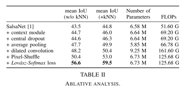
D. Ablation Study
In this ablation analysis, we investigate the individual contribution of each improvement to the original SalsaNet model. Table II shows the model parameters and the total number of FLOPs (floating point operations) for mIoU scores obtained on the Semantic-KITTI test set before and after applying kNN-based post-processing (see Section III-F).
As shown in Table II, each of our contributions on SalsaNet has a unique improvement in accuracy. The post-processing step leads to a certain jump in accuracy (about 2%). A spike in model parameters was observed when dilated convolutional stacks were introduced in the encoder, which was greatly reduced after adding a pixel shuffling layer in the decoder. Combining weighted cross-entropy loss with Lov'asz-Softmax gives the highest increase in accuracy due to the direct optimization of the Jaccard exponent. Compared with the original SalsaNet model, we can achieve the highest accuracy score of 59.5% with only 2.2% (i.e. 0.15M) extra parameters. Table II also shows that the number of FLOPs is related to the number of parameters. We note that adding knowledge and arbitrary uncertainty computations does not introduce any additional training parameters, since they are computed after the network is trained.
E. Runtime Evaluation
Runtime performance is critical in autonomous driving. Table III reports the aggregate runtime performance of SalsaNext's CNN backbone and post-processing modules compared to other networks. In order to obtain fair statistics, all measurements were performed using the entire Semantic-KITTI dataset on the same NVIDIA Quadro RTX 6000 - 24 GB card. As shown in Table III, our method shows significantly better performance compared to RangeNet++ [7] while having 7 times more parameters. SalsaNext can run at 24 Hz when uncertain calculations are excluded for fair comparison with deterministic models. Note that this high speed we achieve is significantly faster than the sampling rate of mainstream LiDAR sensors, which typically operate at 10 Hz [39]. Figure 1 also compares the overall performance of SalsaNext with other state-of-the-art semantic segmentation networks in terms of runtime, accuracy, and memory consumption.
5 Conclusion
We propose a new uncertainty-aware semantic segmentation network, named SalsaNext, which can process full 360◦ LiDAR scans in real-time. SalsaNext builds on the SalsaNet model and can achieve an accuracy rate of over 14%. Compared to previous methods, SalsaNext returns +3.6% higher mIoU scores. Our approach differs in that SalsaNext also estimates data and model-based uncertainties.
Summarize yourself:
I took a rough look, but I didn’t look very carefully. I feel that everyone’s network structure looks similar. This is the processing network of the lidar stream in pmf, so I took a rough look. The innovation point should be the measurement of uncertainty and real-time performance.