Deep Learning with Python: Neural Networks (full tutorial) Build, graph, and interpret artificial neural networks using TensorFlow
Summarize
In this article, I show how to build neural networks using Python, and how to explain deep learning to business using visualization and creating model predictive explainers.
Image credit: Author Deep learning, a type of machine learning that mimics the way humans acquire certain types of knowledge, has grown in popularity over the years compared to standard models.
While traditional algorithms are linear, deep learning models (often neural networks) are stacked in an increasingly complex and abstract hierarchy (hence the "depth" in deep learning).
Neural networks are based on a group of connected units (neurons), which, like synapses in the brain, can transmit signals to other neurons, so that, like interconnected brain cells, they can communicate in a more human-like manner. Learn and make decisions.
Today, deep learning is so popular that many companies want to use it, even if they don't fully understand it. Often, data scientists first have to simplify these complex algorithms for the business and then explain and justify the model's results, which is not always so simple with neural networks. I think the best way is through visualization.
I'll introduce some useful Python code that can be easily applied to other similar situations (just copy, paste, run), and walk through each line of code with comments so you can replicate the examples.
In particular, I will go through:
Environment settings, tensorflow and pytorch
Artificial Neural Network Segmentation, Input, Output, Hidden Layers, Activation Functions
Deep Learning with Deep Neural Networks
Model design with tensorflow/keras
Visualize neural networks using python
Model training and testing
explained by shape
set up
There are two main libraries for building neural networks: TensorFlow (developed by Google) and PyTorch (developed by Facebook). They can perform similar tasks, but the former is more suitable for production, while the latter is suitable for building rapid prototypes because it is easier to learn.
These two libraries are favored by the community and enterprises because they can take advantage of the power of NVIDIA GPUs. This is useful, and sometimes even necessary, for working with large datasets such as text corpora or image libraries.
在本教程中,我将使用 TensorFlow 和 Keras,这是一个比纯 TensorFlow 和 PyTorch 更用户友好的更高级别的模块,尽管速度有点慢。
第一步是通过终端安装 TensorFlow:
pip install tensorflow 如果要启用GPU支持,可以阅读官方文档或遵循本指南。设置完成后,您的 Python 指令将由您的机器转换为 CUDA 并由 GPU 处理,因此您的模型将运行得非常快。
现在我们可以在笔记本上导入 TensorFlow Keras 的主要模块并开始编码:
from tensorflow.keras import models, layers, utils, backend as K
import matplotlib.pyplot as plt
import shap
人工神经网络
ANN由具有输入和输出维度的层组成。后者由神经元(也称为“节点”)的数量决定,神经元是一个计算单元,通过激活函数连接加权输入(帮助神经元打开/关闭)。
与大多数机器学习算法一样,权重在训练期间随机初始化和优化,以最小化损失函数。
图层可以分组为:
输入层具有将输入向量传递给神经网络的工作。如果我们有一个包含 3 个特征的矩阵(形状 N x 3),则该层将 3 个数字作为输入,并将相同的 3 个数字传递给下一层。
隐藏层代表中间节点,它们对数字进行多次转换以提高最终结果的准确性,输出由神经元的数量定义。
返回神经网络最终输出的输出层。如果我们在做一个简单的二元分类或回归,输出层应该只有 1 个神经元(因此它只返回 1 个数字)。
在具有 5 个不同类的多类分类的情况下,输出层应具有 5 个神经元。
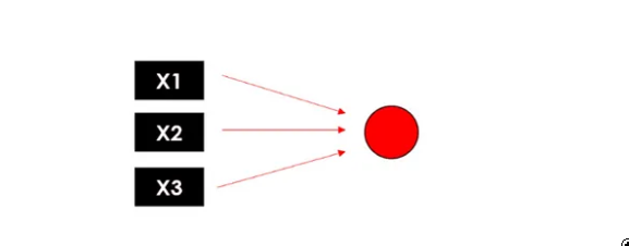
ANN最简单的形式是感知器,一个只有一层的模型,与线性回归模型非常相似。询问感知器内部发生了什么,相当于询问多层神经网络的单个节点内部发生了什么......让我们分解一下。
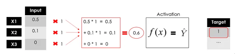
假设我们有一个包含 N 行、3 个特征和 1 个目标变量(即二进制 1/0)的数据集:
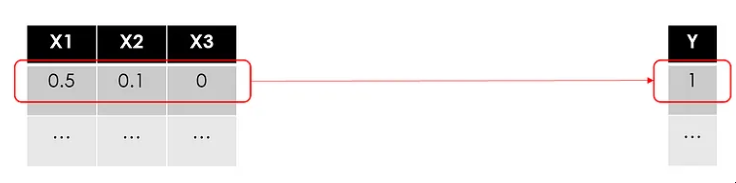
我在 0 到 1 之间放置了一些随机数数据在输入神经网络之前应始终缩放。
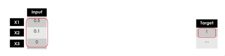
就像在所有其他机器学习用例中一样,我们将训练一个模型来逐行使用特征预测目标。让我们从第一行开始:
“训练模型”是什么意思?
在数学公式中搜索最佳参数,以最大程度地减少预测误差。在回归模型,即线性回归中,您必须找到最佳权重,在基于树的模型(即随机森林)中,这是关于找到最佳拆分点......
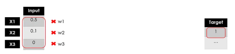
通常,权重是随机初始化的,然后随着学习的进行进行调整。在这里,我将它们全部设置为 1:
图片来源:作者
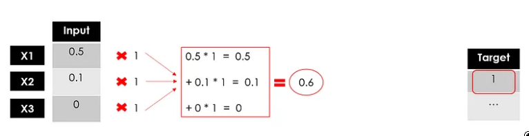
到目前为止,我们还没有做任何与线性回归不同的事情。对于业务来说,这很简单。
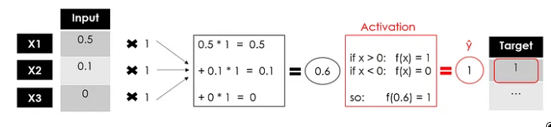
现在,这里是从线性模型 Σ(xiwi)=Y 到非线性模型 f ( Σ(xiwi)=Y 的升级...输入激活函数。
图片来源:作者
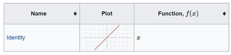
激活函数定义该节点的输出。有很多,甚至可以创建一些自定义函数,您可以在官方文档中找到详细信息并查看此备忘单。如果我们在示例中设置一个简单的线性函数,那么我们与线性回归模型没有区别。
来源:维基百科
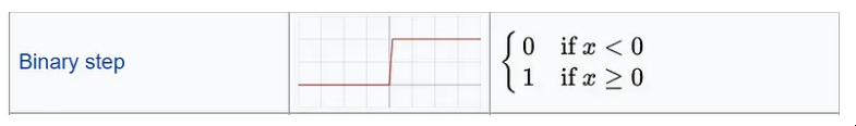
我将使用仅返回 1 或 0 的二进制步骤激活函数:
来源:维基百科
图片来源:作者
我们有感知器的输出,这是一个单层神经网络,它接受一些输入并返回 1 个输出。现在,模型的训练将继续,将输出与目标进行比较,计算误差并优化权重,一次又一次地重复整个过程。
图片来源:作者 这是神经元的常见表示形式:
图片来源:作者
深度神经网络
可以说所有的深度学习模型都是神经网络,但并非所有的神经网络都是深度学习模型。一般来说,“深度”学习适用于算法至少有 2 个隐藏层(因此总共 4 层,包括输入和输出)的情况。
想象一下同时复制神经元进程3次:由于每个节点(加权和和激活函数)返回一个值,我们将拥有具有3个输出的第一个隐藏层。
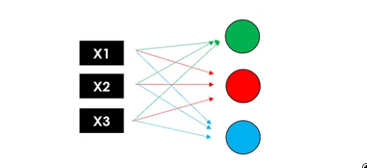
图片来源:作者 现在让我们再次使用这 3 个输出作为第二个隐藏层的输入,该隐藏层返回 3 个新数字。最后,我们将添加一个输出层(仅 1 个节点)以获得模型的最终预测。
图片来源:作者 请记住,这些层可以具有不同数量的神经元和不同的激活函数,并且在每个节点中,权重被训练以优化最终结果。这就是为什么添加的层越多,可训练参数的数量就越多。
现在,您可以查看神经网络的全貌:
图片来源:作者 请注意,为了尽可能简单,我没有提到业务部门可能不感兴趣的某些细节,但数据科学家绝对应该意识到这一点。特别:
偏差:在每个神经元内部,输入和权重的线性组合还包括一个偏差,类似于线性方程中的常数,因此神经元的完整公式为 f( Σ(Xi * Wi ) + 偏置 )
反向传播:在训练期间,模型通过将误差传播回节点并更新参数(权重和偏差)来学习,以最大程度地减少损失。
来源:3Blue1Brown (Youtube) 梯度下降:用于训练神经网络的优化算法,通过在最陡下降的方向上重复步骤来找到损失函数的局部最小值。
source: 3Blue1Brown (Youtube)
Model Design
The easiest way to build a Neural Network with TensorFlow is with the Sequential class of Keras. Let’s use it to make the Perceptron from our previous example, so a model with only one Dense layer. It is the most basic layer as it feeds all its inputs to all the neurons, each neuron providing one output.
model = models.Sequential(name="Perceptron", layers=[
layers.Dense( #a fully connected layer
name="dense",
input_dim=3, #with 3 features as the input
units=1, #and 1 node because we want 1 output
activation='linear' #f(x)=x
)
])
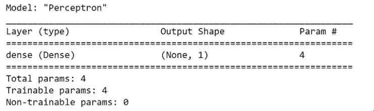
model.summary()

图片来源:作者
摘要函数提供结构和大小的快照(就要训练的参数而言)。在这种情况下,我们只有 4 个(3 个权重和 1 个偏差),所以它非常轻巧。
如果你想使用Keras中尚未包含的激活函数,就像我在可视化示例中展示的二进制步骤函数一样,你必须弄脏原始TensorFlow:
# define the function
import tensorflow as tf
def binary_step_activation(x):
    ##return 1 if x>0 else 0
    return K.switch(x>0, tf.math.divide(x,x), tf.math.multiply(x,0))

# build the model
model = models.Sequential(name="Perceptron", layers=[
      layers.Dense(
          name="dense",
          input_dim=3,
          units=1,
          activation=binary_step_activation
      )
])
现在让我们尝试从感知器转向深度神经网络。可能你会问自己一些问题:
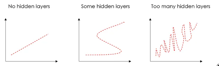
多少层? 正确的答案是“尝试不同的变体,看看什么有效”。
我通常使用 Dropout 处理 2 个密集隐藏层,这是一种通过将输入随机设置为 0 来减少过度拟合的技术。
隐藏层对于克服数据的非线性很有用,因此如果您不需要非线性,则可以避免隐藏层。过多的隐藏层会导致过度拟合。
图片来源:作者
有多少神经元? 隐藏神经元的数量应该介于输入层的大小和输出层的大小之间。我的经验法则是(输入数 + 1 输出)/2。
什么是激活功能? 有很多,我们不能说一个绝对更好。无论如何,最常用的是 ReLU,这是一个分段线性函数,只有在为正时才返回输出,并且主要用于隐藏层。
此外,输出层必须具有与预期输出兼容的激活。例如,线性函数适用于回归问题,而 Sigmoid 通常用于分类。
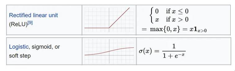
来源:维基百科
我将假设一个包含 N 个特征和 1 个二进制目标变量的输入数据集(很可能是一个分类用例)。
n_features = 10
model = models.Sequential(name="DeepNN", layers=[
    ### hidden layer 1
    layers.Dense(name="h1", input_dim=n_features,
                 units=int(round((n_features+1)/2)),
                 activation='relu'),
    layers.Dropout(name="drop1", rate=0.2),

    ### hidden layer 2
    layers.Dense(name="h2", units=int(round((n_features+1)/4)),
                 activation='relu'),
    layers.Dropout(name="drop2", rate=0.2),

    ### layer output
    layers.Dense(name="output", units=1, activation='sigmoid')
])
model.summary()
图片来源:作者
请注意,顺序类并不是使用 Keras 构建神经网络的唯一方法。Model 类提供了对层的更大灵活性和控制,可用于构建具有多个输入/输出的更复杂的模型。有两个主要区别:
在顺序类中,需要指定输入层,它隐含在第一个密集层的输入维度中。 这些图层像对象一样保存,可以应用于其他图层的输出,例如:输出 = layer(...)(输入) 这就是如何使用 Model 类来构建我们的感知器和 DeepNN:
# Perceptron
inputs = layers.Input(name="input", shape=(3,))
outputs = layers.Dense(name="output", units=1,
                       activation='linear')(inputs)
model = models.Model(inputs=inputs, outputs=outputs,
                     name="Perceptron")

# DeepNN
### layer input
inputs = layers.Input(name="input", shape=(n_features,))
### hidden layer 1
h1 = layers.Dense(name="h1", units=int(round((n_features+1)/2)), activation='relu')(inputs)
h1 = layers.Dropout(name="drop1", rate=0.2)(h1)
### hidden layer 2
h2 = layers.Dense(name="h2", units=int(round((n_features+1)/4)), activation='relu')(h1)
h2 = layers.Dropout(name="drop2", rate=0.2)(h2)
### layer output
outputs = layers.Dense(name="output", units=1, activation='sigmoid')(h2)
model = models.Model(inputs=inputs, outputs=outputs, name="DeepNN")
始终可以检查模型摘要中的参数数量是否与顺序中的参数数量相同。
可视化
请记住,我们正在向企业讲述一个故事,可视化是我们最好的盟友。
我准备了一个函数来绘制人工神经网络的 TensorFlow 模型的结构,这是完整的代码:
'''
Extract info for each layer in a keras model.
'''
def utils_nn_config(model):
    lst_layers = []
    if "Sequential" in str(model): #-> Sequential doesn't show the input layer
        layer = model.layers[0]
        lst_layers.append({

    "name":"input", "in":int(layer.input.shape[-1]), "neurons":0,
                           "out":int(layer.input.shape[-1]), "activation":None,
                           "params":0, "bias":0})
    for layer in model.layers:
        try:
            dic_layer = {

    "name":layer.name, "in":int(layer.input.shape[-1]), "neurons":layer.units,
                         "out":int(layer.output.shape[-1]), "activation":layer.get_config()["activation"],
                         "params":layer.get_weights()[0], "bias":layer.get_weights()[1]}
        except:
            dic_layer = {

    "name":layer.name, "in":int(layer.input.shape[-1]), "neurons":0,
                         "out":int(layer.output.shape[-1]), "activation":None,
                         "params":0, "bias":0}
        lst_layers.append(dic_layer)
    return lst_layers


'''
Plot the structure of a keras neural network.
'''
def visualize_nn(model, description=False, figsize=(10,8)):
    ## get layers info
    lst_layers = utils_nn_config(model)
    layer_sizes = [layer["out"] for layer in lst_layers]

    ## fig setup
    fig = plt.figure(figsize=figsize)
    ax = fig.gca()
    ax.set(title=model.name)
    ax.axis('off')
    left, right, bottom, top = 0.1, 0.9, 0.1, 0.9
    x_space = (right-left) / float(len(layer_sizes)-1)
    y_space = (top-bottom) / float(max(layer_sizes))
    p = 0.025

    ## nodes
    for i,n in enumerate(layer_sizes):
        top_on_layer = y_space*(n-1)/2.0 + (top+bottom)/2.0
        layer = lst_layers[i]
        color = "green" if i in [0, len(layer_sizes)-1] else "blue"
        color = "red" if (layer['neurons'] == 0) and (i > 0) else color

        ### add description
        if (description is True):
            d = i if i == 0 else i-0.5
            if layer['activation'] is None:
                plt.text(x=left+d*x_space, y=top, fontsize=10, color=color, s=layer["name"].upper())
            else:
                plt.text(x=left+d*x_space, y=top, fontsize=10, color=color, s=layer["name"].upper())
                plt.text(x=left+d*x_space, y=top-p, fontsize=10, color=color, s=layer['activation']+" (")
                plt.text(x=left+d*x_space, y=top-2*p, fontsize=10, color=color, s="Σ"+str(layer['in'])+"[X*w]+b")
                out = " Y"  if i == len(layer_sizes)-1 else " out"
                plt.text(x=left+d*x_space, y=top-3*p, fontsize=10, color=color, s=") = "+str(layer['neurons'])+out)

        ### circles
        for m in range(n):
            color = "limegreen" if color == "green" else color
            circle = plt.Circle(xy=(left+i*x_space, top_on_layer-m*y_space-4*p), radius=y_space/4.0, color=color, ec='k', zorder=4)
            ax.add_artist(circle)

            ### add text
            if i == 0:
                plt.text(x=left-4*p, y=top_on_layer-m*y_space-4*p, fontsize=10, s=r'$X_{'+str(m+1)+'}$')
            elif i == len(layer_sizes)-1:
                plt.text(x=right+4*p, y=top_on_layer-m*y_space-4*p, fontsize=10, s=r'$y_{'+str(m+1)+'}$')
            else:
                plt.text(x=left+i*x_space+p, y=top_on_layer-m*y_space+(y_space/8.+0.01*y_space)-4*p, fontsize=10, s=r'$H_{'+str(m+1)+'}$')

    ## links
    for i, (n_a, n_b) in enumerate(zip(layer_sizes[:-1], layer_sizes[1:])):
        layer = lst_layers[i+1]
        color = "green" if i == len(layer_sizes)-2 else "blue"
        color = "red" if layer['neurons'] == 0 else color
        layer_top_a = y_space*(n_a-1)/2. + (top+bottom)/2. -4*p
        layer_top_b = y_space*(n_b-1)/2. + (top+bottom)/2. -4*p
        for m in range(n_a):
            for o in range(n_b):
                line = plt.Line2D([i*x_space+left, (i+1)*x_space+left],
                                  [layer_top_a-m*y_space, layer_top_b-o*y_space],
                                  c=color, alpha=0.5)
                if layer['activation'] is None:
                    if o == m:
                        ax.add_artist(line)
                else:
                    ax.add_artist(line)
    plt.show()
让我们在我们的 2 个模型上尝试一下,首先是感知器:
visualize_nn(model, description=True, figsize=(10,8))
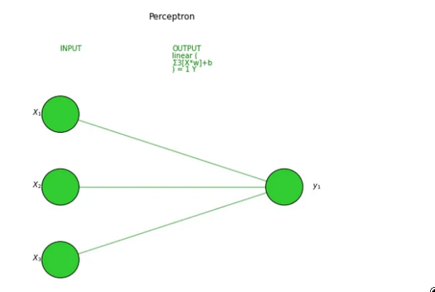
图片来源:作者
然后是深度神经网络:
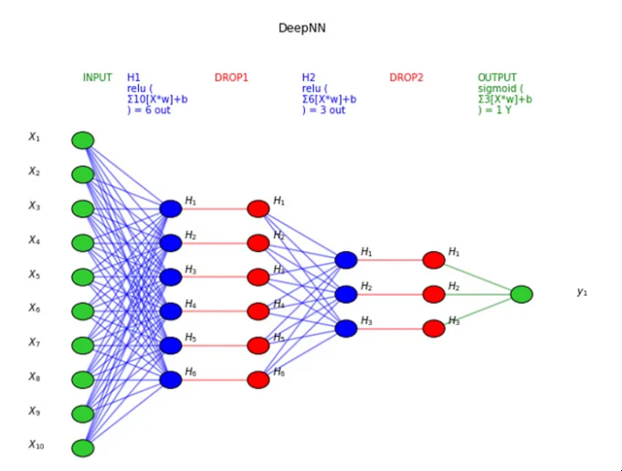
图片来源:作者
TensorFlow也提供了一个绘制模型结构的工具,你可能希望将其用于具有更复杂层(CNN,RNN等)的更复杂的神经网络。有时设置起来有点棘手,如果您有问题,这篇文章可能会有所帮助。
utils.plot_model(model, to_file='model.png', show_shapes=True, show_layer_names=True)
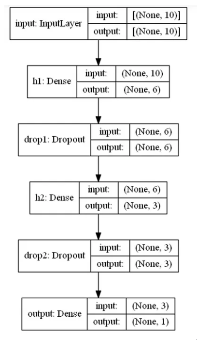
图片来源:作者
这会将此图像保存在笔记本电脑上,因此,如果您只想将其绘制在笔记本上,只需运行以下命令即可删除该文件:
import os
os.remove('model.png')
训练与测试
最后,是时候训练我们的深度学习模型了。为了使它运行,我们必须“编译”,或者换句话说,我们需要定义优化器、损失函数和指标。
我通常使用 Adam 优化器,这是一种梯度下降的替代优化算法(自适应优化器中最好的)。其他参数取决于用例。
在(二元)分类问题中,您应该使用(二元)交叉熵损失,它将每个预测概率与实际类输出进行比较。
至于指标,我喜欢监控准确性和 F1 分数,这是一个结合了精度和召回率的指标(后者必须实现,因为它尚未包含在 TensorFlow 中)。
# define metrics
def Recall(y_true, y_pred):
    true_positives = K.sum(K.round(K.clip(y_true * y_pred, 0, 1)))
    possible_positives = K.sum(K.round(K.clip(y_true, 0, 1)))
    recall = true_positives / (possible_positives + K.epsilon())
    return recall

def Precision(y_true, y_pred):
    true_positives = K.sum(K.round(K.clip(y_true * y_pred, 0, 1)))
    predicted_positives = K.sum(K.round(K.clip(y_pred, 0, 1)))
    precision = true_positives / (predicted_positives + K.epsilon())
    return precision

def F1(y_true, y_pred):
    precision = Precision(y_true, y_pred)
    recall = Recall(y_true, y_pred)
    return 2*((precision*recall)/(precision+recall+K.epsilon()))

# compile the neural network
model.compile(optimizer='adam', loss='binary_crossentropy',
              metrics=['accuracy',F1])
另一方面,在回归问题中,我通常将 MAE 设置为损失,将 R 平方设置为度量。
# define metrics
def R2(y, y_hat):
    ss_res =  K.sum(K.square(y - y_hat))
    ss_tot = K.sum(K.square(y - K.mean(y)))
    return ( 1 - ss_res/(ss_tot + K.epsilon()) )

# compile the neural network
model.compile(optimizer='adam', loss='mean_absolute_error',
              metrics=[R2])
在开始训练之前,我们还需要确定 Epochs 和 Batches:由于数据集可能太大而无法一次全部处理,因此将其拆分为多个批次(批处理大小越大,需要的内存空间就越多)。
反向传播和随后的参数更新每批发生一次,是整个训练集的一次传递。因此,如果您有 100 个观测值,并且批大小为 20,则需要 5 个批次才能完成 1 个 epoch。批大小应为 2 的倍数(常见:32、64、128、256),因为计算机通常以 2 的幂组织内存。
我倾向于从 100 个 epoch 开始,批大小为 32。
在训练期间,我们希望看到指标得到改善,损失逐个时期减少。此外,最好保留一部分数据 (20%-30%) 进行验证。
换句话说,模型将分离这部分数据,以评估训练之外的每个纪元结束时的损失和指标。
假设你已经把你的数据准备好到一些 X 和 y 数组中(如果没有,你可以简单地生成随机数据,如
import numpy as np
X = np.random.rand(1000,10)
y = np.random.choice([1,0], size=1000)
),您可以按如下方式启动和可视化训练:

# train/validation
training = model.fit(x=X, y=y, batch_size=32, epochs=100, shuffle=True, verbose=0, validation_split=0.3)

# plot
metrics = [k for k in training.history.keys() if ("loss" not in k) and ("val" not in k)]
fig, ax = plt.subplots(nrows=1, ncols=2, sharey=True, figsize=(15,3))

## training
ax[0].set(title="Training")
ax11 = ax[0].twinx()
ax[0].plot(training.history['loss'], color='black')    ax[0].set_xlabel('Epochs')
ax[0].set_ylabel('Loss', color='black')
for metric in metrics:
    ax11.plot(training.history[metric], label=metric)    ax11.set_ylabel("Score", color='steelblue')
ax11.legend()

## validation
ax[1].set(title="Validation")
ax22 = ax[1].twinx()
ax[1].plot(training.history['val_loss'], color='black')    ax[1].set_xlabel('Epochs')
ax[1].set_ylabel('Loss', color='black')
for metric in metrics:
    ax22.plot(training.history['val_'+metric], label=metric)    ax22.set_ylabel("Score", color="steelblue")
plt.show()
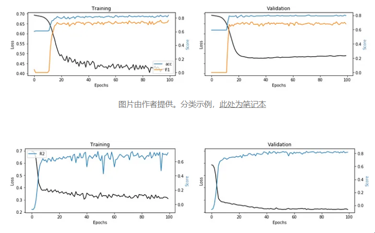
图片由作者提供分类示例
图片由作者提供。回归示例,此处为笔记本 这些图取自两个实际用例,这两个用例将标准机器学习算法与神经网络进行比较(每个图像下的链接)。
可解释性
我们训练并测试了我们的模型,但我们仍然没有说服业务部门相信结果......我们能做什么?很简单,我们构建了一个解释器来证明我们的深度学习模型不是一个黑匣子。
我发现Shap与神经网络配合得很好:对于每个预测,它能够估计每个特征对模型预测值的贡献。基本上,它回答了“为什么模型说这是 1 而不是 0?”的问题。
您可以使用以下代码:
请注意,您也可以在其他机器学习模型(即线性回归、随机森林)上使用此功能,而不仅仅是神经网络。
正如您可以从代码中读到的那样,如果X_train参数保留为 None,我的函数假定它不是深度学习。
让我们在分类和回归示例中对其进行测试:
i = 1
explainer_shap(model,
               X_names=list_feature_names,
               X_instance=X[i],
               X_train=X,
               task="classification", #task="regression"
               top=10)
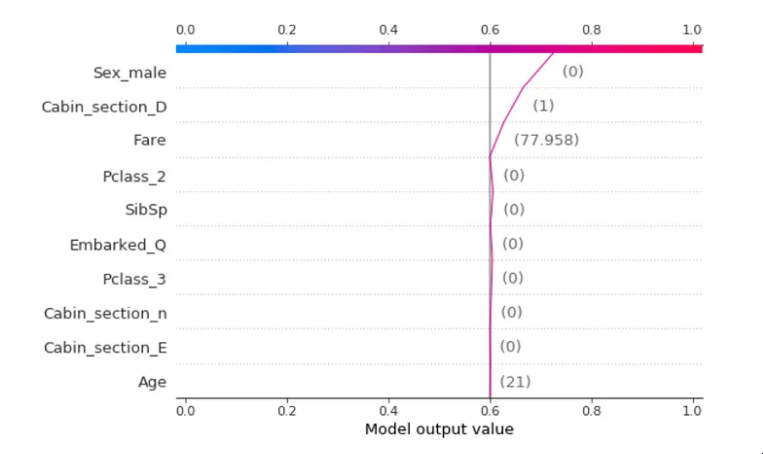
图片由作者提供。分类示例,泰坦尼克号数据集中,预测是“幸存”主要是因为虚拟变量_male=0,所以乘客是女性。
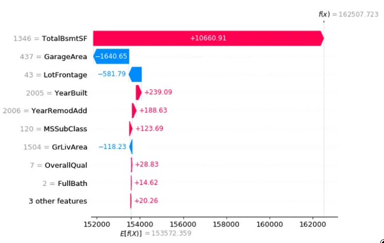
图片由作者提供。回归示例房价数据集,这个房价的主要驱动力是一个大地下室。
结论
本文是一个教程,演示如何设计和构建人工神经网络,无论是深度的还是非深度的。 我一步一步地分解了单个神经元内部发生的事情,更普遍地说是层内发生的事情。我让这个故事变得简单,就好像我们正在向业务部门解释深度学习一样,使用了大量的可视化。
在本教程的第二部分中,我们使用TensorFlow创建了一些神经网络,从感知器到更复杂的神经网络。然后,我们训练了深度学习模型,并评估了它在分类和回归用例中的可解释性。
本文由 mdnice 多平台发布