Mathematical Modeling: Predictive Model Learning - Gray Predictive Model (GM(1,1) Model)

Table of contents

foreword

1. Model realization

1. Process introduction

2. Gray generation

1. Accumulation generation operator

 2. Mean generating operator

3. Feasibility analysis (gradation test)

4. Establish GM(1,1) model

1. Data preprocessing:

 2. Build a model:

3. Construct data matrix B and data vector Y:

5. Accuracy inspection

2. Case Analysis

Summarize

---

foreword

Briefly introduce the gray forecasting model, and use matlab to analyze specific cases, and will continue to add later

---

1. Model realization

1. Process introduction

• Gray generates new operators
• Feasibility Analysis
• Build a GM(1,1) model
• precision test

2. Gray generation

To put it simply, the purpose of the gray generation new operator is to weaken the randomness of the disordered sequence and transform it into an ordered sequence to show the rules and analyze it. The common generation operators are as follows:

• 1. Accumulative Generation Operator (AGO)
• 2. Inverse accumulative generation operator (IAGO)
• 3. Mean generation operator (MEAN)
• 4. Scale generation operator

1. Accumulation generation operator

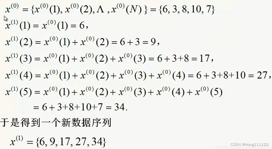
The line graph of the new sequence and the old sequence is as follows. It can be seen that the new sequence converts the original irregular sequence into a clearly regular and increasing sequence:

 

 2. Mean generating operator

That is, calculate the average value of the adjacent two items of the cumulative generating operator , taking the above example as an example:

3. Feasibility analysis (gradation test)

First calculate the ratio of each item of the original sequence , that is, the ratio, taking the above example as an example:

Calculated grade ratio:     

If the grade ratio is satisfied:

 Then the new operator may establish a GM(1,1) model

ps: There is a condition that it must be non- negative. If there is a negative number item, add a positive number a after it so that  the and or are both non-negative before performing subsequent operations.       

4. Establish GM(1,1) model

1. Data preprocessing:

Assume first that the original sequence passes the grade test,

Take the mean generating operator as an example:

New order: 

ps: Similarly, if the grade ratio test fails, a positive number a can also be added after it , so that all grade ratios are within the allowable range.

 2. Build a model:

1. Original form:     , purpose: find out a, b

2. Estimate a, b by regression analysis, the corresponding whitening differential equation and its solution are:

 From this we get the predicted value:

 Original sequence prediction value:

3. Construct data matrix B and data vector Y:

                    

So    , solving the above differential equation, we get 

Calculate a, b and substitute the above predicted value to fit a predicted value function

5. Accuracy inspection

Residual test:

If the absolute value of all residuals is less than 0.1, it is considered to meet the higher requirements; if it is less than 0.2, it meets the general requirements;

Scale deviation test:

 If the absolute value of all grade ratio deviations is less than 0.1, it is considered to meet the higher requirements; if it is less than 0.2, it meets the general requirements;

2. Case Analysis

Predict the number of permanent residents in the next n years based on the number of permanent residents in Fujian Province in the past ten years

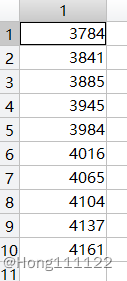
2010--2020 data: [3693,3784,3841,3885,3945,3984,4016,4065,4104,4137,4161] million people

1. Grade ratio test: 

        Meet the grade ratio test interval: (0.8574, 1.1663)

The grade ratio calculated by matlab is:

Passed the grade test

code:

%级比检验通过
check = [];
for k = 2:n
    lambda(k) = data(k-1)/data(k);
    if (exp(-2/(n+1))<lambda(k))&&(lambda(k)<exp(2/(n+1)))
        check(end+1) = 1;  %通过则输出1
    else check(end+1) = 0;  %不通过则输出0
    end
end 

2. Generate operator:

 Cumulative generation operator:

Mean generating operator:

code:

%累加生成算子
X1 = cumsum(data);
for i=2:n
    z(i) = 0.5*(X1(i-1)+X1(i));
end

3. Find the data matrix B and data vector Y

B：                                                                                               Y：

                                                      

code:

%数据矩阵B及数据向量Y
Y = data(2:n)';
B = [-z(2:n)',ones(n-1,1)];
u = (B'*B)\B'*Y;
a = u(1,1);
b = u(2,1);

4. Generate predictions and

： 

 ：

code:

%预测值
f_X1 = [];
f_X0 = [];
for k=1:n-1
    f_X1(1)=data(1);
    f_X1(k+1) = (data(1)-b/a)*exp(-a*k) + b/a;
end
for k=2:n
    f_X0(1)=data(1);
    f_X0(k)=f_X1(k)-f_X1(k-1);
end

5. Residual error test and scale deviation test:

Residual test:

  Scale deviation test: 

Both are less than 0.1, which proves that the model has high accuracy and can be used for prediction

 code:

%残差检验&级比偏差值检验
for k=1:n-1
    sigma(k)=abs((data(k)-f_f_X0(k))/data(k));
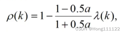
    rho(k+1)=abs(1-((1-0.5*a)*lambda(k+1))/(1+0.5*a));
end

 6. The complete code is as follows, you need to predict how much you can input by yourself:

%10至20年数据，21年数据为4219
data = [3693,3784,3841,3885,3945,3984,4016,4065,4104,4137,4161];
n = length(data);

%级比检验通过
check = [];
for k = 2:n
    lambda(k) = data(k-1)/data(k);
    if (exp(-2/(n+1))<lambda(k))&&(lambda(k)<exp(2/(n+1)))
        check(end+1) = 1;
    else check(end+1) = 0;
    end
end 

%累加生成算子
X1 = cumsum(data);
for i=2:n
    z(i) = 0.5*(X1(i-1)+X1(i));
end

%数据矩阵B及数据向量Y
Y = data(2:n)';
B = [-z(2:n)',ones(n-1,1)];
u = (B'*B)\B'*Y;
a = u(1,1);
b = u(2,1);

%预测值
f_X1 = [];
f_X0 = [];
for k=1:n-1
    f_X1(1)=data(1);
    f_X1(k+1) = (data(1)-b/a)*exp(-a*k) + b/a;
end
for k=2:n
    f_X0(1)=data(1);
    f_X0(k)=f_X1(k)-f_X1(k-1);
end

%残差检验&级比偏差值检验
for k=1:n-1
    sigma(k)=abs((data(k)-f_f_X0(k))/data(k));
    rho(k+1)=abs(1-((1-0.5*a)*lambda(k+1))/(1+0.5*a));
end

%预测下n个值
test = input('nums:');
n=n+test;
f_f_X1 = [];
f_f_X0 = [];
for k=1:n-1
    f_f_X1(1)=data(1);
    f_f_X1(k+1) = (data(1)-b/a)*exp(-a*k) + b/a;
end
for k=2:n
    f_f_X0(1)=data(1);
    f_f_X0(k)=f_f_X1(k)-f_f_X1(k-1);
end

 As a result, the 21-year resident population is 42.28 million, which is close to the real data of 4219.

3. Analysis and summary