Hands-on data analysis records

This article was first published on the knowledge planet check-in content ( BrainTechnology Planet ), and all links in this article are accessed through blogs.

The learning in this article is mainly for the use of punch-in content, not a tutorial course.

Source of this learning tutorial: https://gitee.com/datawhalechina/hands-on-data-analysis

Task arrangement for this content

Task01: Data loading and exploratory data analysis (2 days)

• Understanding Data Loading and Data Observation
• Master pandas basics
• Complete exploratory data analysis

The main learning content is : Chapter 123 of the course

Task02: Data cleaning and feature processing (2 days)

• Master the method of data cleaning
• Understanding Feature Observation and Processing

The main learning content is : Part 1 of the second chapter of the course (data cleaning and feature processing)

Task03: Data reconstruction (2 days)

• Learn about data reconstruction methods
• Use groupby to do data operations

The main learning content is : Chapter 2, Part 2 and Part 3 of the course (data reconstruction)

Task04: Data visualization (2 days)

• Understand the purpose of visualization
• Know the scenarios in which various graphics can be used
• The basic library of actual data visualization

The main learning content is : Chapter 2, Part 4 of the course (Data Visualization)

Task05: Data modeling and model evaluation (2 days)

• Learn about data modeling
• Use sklearn to complete the modeling of the classification model
• Learn about model evaluation
• Model evaluation is done using sklearn

The main learning content is : Chapter 3 of the course (data modeling and model evaluation)

This study is arranged according to the course outline and will be completed from September 12, 2021 to September 22, 2021

The following content is punch card learning content:

First of all, you need some prior knowledge before learning, know a little about the use of Python and pandas, you can refer to the website of learning aids: http://joyfulpandas.datawhale.club/Content/ch1.html

Task 00 Install jupyter and be familiar with the above URL

The computer I am currently using is a MacBook Pro, so I only need to install anaconda and it will come with Jupyter. In the terminal, I can enter jupyter notebook / jupyter-notebook or python3 -m IPython notebook to open it

Preparation materials content: Chapter 6 of the book "Python for Data Analysis"

Task 01 Data loading and exploratory data analysis

Chapter 1 Section 1

#数据集下载https://www.kaggle.com/c/titanic/overview
#第一步导入numpy和pandas
import numpy as np
import pandas as pd

#第二步加载数据
#相对路径
df = pd.read_csv('train.csv')
df.head(3)
#绝对路径
df = pd.read_csv('/Users/chenrui/Desktop/hands-on-data-analysis-master/第一单元项目集合/train.csv')
df.head(3)

#尝试使用os.getcwd()查看当前工作路径时，需要先import os

#第三步逐块读取
chunker = pd.read_csv('train.csv',chunksize = 1000)
#思考：什么是逐块读取？为什么要逐块读取呢？
#设置chunksize参数，来控制每次迭代数据的大小
chunker = pd.read_csv("train.csv",chunksize=1000)
for piece in chunker:
    print(type(piece))
    #<class 'pandas.core.frame.DataFrame'>
    print(len(piece))
    #891

#第四步将表头改成中文
df = pd.read_csv('train.csv', names=['乘客ID','是否幸存','仓位等级','姓名','性别','年龄','兄弟姐妹个数','父母子女个数','船票信息','票价','客舱','登船港口'],index_col='乘客ID',header=0)
df.head()

#查看数据基本信息
df.info()

#查看表格前十行和后15行数据
df.head(10)
df.tail(15)

#判断数据是否为空,判断数据是否为空，为空的地方返回True，其余地方返回False
df.isnull().head()
#思考：对于一个数据，还可以从哪些方面来观察？
df.describe()
#获取每列数据的统计特征
# .describe()即可查看每列数据
'''
（1）总行数统计count
（2）平均值mean
（3）标准差std
（4）最小值min
（5）25%分位值“25%”
（6）50%分位值“50%”
（7）75%分位值“75%”
（8）最大值max
'''

#保存数据
df.to_csv('train_test.csv')

Chapter 1 Section 2

Know the data and understand the meaning of the data fields

#任务一：pandas中有两个数据类型DateFrame和Series
#series:类似于1维数组，由索引+数值组成
#dataframe是非常常见的一个表格型数据结构，每一列可以是不同的数值类型，有行索引、列索引。提到它就会自然想到Pandas这个包。平常用Python处理xlsx、csv文件，读出来的就是dataframe格式。
#参考链接：https://zhuanlan.zhihu.com/p/41092771

#加载库
import numpy as np
import pandas as pd

#Series的展示
sdata = {
    
    '0hio':35000,'Texas':71000,'0regon':16000,'Utah':5000}
example_1 = pd.Series(sdata)
example_1

#DataFrame的展示
data = {
    
    'state': ['Ohio', 'Ohio', 'Ohio', 'Nevada', 'Nevada', 'Nevada'],
        'year': [2000, 2001, 2002, 2001, 2002, 2003],'pop': [1.5, 1.7, 3.6, 2.4, 2.9, 3.2]}
example_2 = pd.DataFrame(data)
example_2


#任务二：加载数据集“train.csv”文件
#使用相对路径加载,并展示前三行数据
df = pd.read_csv('train.csv')
df.head(3)

#任务三：查看DataFrame数据的每列名称
df.columns

#任务四：查看“Cabin”这列数据的所有值
df['Cabin'].head(3) #第一种方法读取

df.Cabin.head(3) #第二种方法读取

#任务五：加载数据集“test_1.csv”,对比train.csv,
test_1 = pd.read_csv('test_1.csv')
test_1.head(3)
#删除多余的列
del test_1['a']
test_1.head(3)

#思考：还有其他的删除多余的列的方式吗？
#使用drop方法进行隐藏,加上参数inplace = True,则将原数据覆盖。
#test_1.drop('a',axis = 1,inplace = True)
test_1.drop('a',axis=1,inplace=True)
test_1.head(3)

#任务六：将【“Passengerld”,"Name","Age","Ticket"】这几个元素隐藏
df.drop(['PassengerId','Name','Age','Ticket'],axis = 1).head(3)

#筛选的逻辑，选出所需要信息，舍弃无用信息。
#任务一：以“Age”为筛选条件，显示年龄在10岁以下的乘客信息
df[df["Age"] < 10].head(3)

#任务二： 以"Age"为条件，将年龄在10岁以上和50岁以下的乘客信息显示出来，并将这个数据命名为midage
midage = df[(df["Age"]>10)& (df["Age"]<50)]
midage.head(3)

#任务三：使用reset_index重置索引，显示数据
midage = midage.reset_index(drop=True)
midage.head(3)

#任务四：使用loc方法将midage数据的第100，105，108行的"Pclass"，"Name"和"Sex"的数据显示出来
midage.loc[[100,105,108],['Pclass','Name','Sex']] 

#任务五：使用iloc方法将midage的数据中第100，105，108行的"Pclass"，"Name"和"Sex"的数据显示出来
midage.iloc[[100,105,108],[2,3,4]]

#思考：对比iloc和loc的异同
#loc函数主要基于行标签和列标签（x_label、y_label）进行索引：使用loc函数，索引的是字符串。
#iloc函数主要基于行索引和列索引（index，columns） 都是从 0 开始：而且，iloc函数索引的数据是int整型，因此是Python默认的前闭后开。注意只能说int型，也就是数字，输入字符的话是会报错的。

Chapter 1 Section 3

Use pandas to sort, calculate and describe the use of describe(). For the content of this section, refer to Chapter 5 of "Using Python for Data Analysis"

#加载库
import numpy as np
import pandas as pd

#载入之前保存的train_chinese.csv数据，关于泰坦尼克号的任务，我们就使用这个数据
text = pd.read_csv('train_chinese.csv')#相对路径
text.head(3)

#任务一：利用pandas进行数据排序，升序
#构建一个都为数字的DataFrame数据
frame = pd.DataFrame(np.arange(8).reshape((2, 4)), 
                     index=['2', '1'], 
                     columns=['d', 'a', 'b', 'c'])
frame
#代码解析
'''
pd.DataFrame() ：创建一个DataFrame对象
np.arange(8).reshape((2, 4)) : 生成一个二维数组（2*4）,第一列：0，1，2，3 第二列：4，5，6，7
index=['2, 1] ：DataFrame 对象的索引列
columns=['d', 'a', 'b', 'c'] ：DataFrame 对象的索引行
'''

# 将构建的DataFrame中的数据根据某一列，升序排列,可以看到sort_values这个函数中by参数指向要排列的列，ascending参数指向排序的方式（升序还是降序）
frame.sort_values(by='c', ascending=True)

# 让行索引升序排序
frame.sort_index()

# 让列索引升序排序
frame.sort_index(axis=1)

# 让列索引降序排序
frame.sort_index(axis=1, ascending=False)

# 让任选两列数据同时降序排序
frame.sort_values(by=['a', 'c'], ascending=False)

#任务二：对train.csv数据按票价和年龄两列进行降序排列，sort_values这个函数中by参数
text.sort_values(by=['票价', '年龄'], ascending=False).head(3)

#任务三：利用pandas进行算术计算，计算两个DataFrame数据
frame1_a = pd.DataFrame(np.arange(9.).reshape(3, 3),
                     columns=['a', 'b', 'c'],
                     index=['one', 'two', 'three'])
frame1_b = pd.DataFrame(np.arange(12.).reshape(4, 3),
                     columns=['a', 'e', 'c'],
                     index=['first', 'one', 'two', 'second'])
frame1_a
frame1_b

#将framel_a和frame_b进行相加
frame1_a + frame1_b

#任务4：计算train.csv中在船上最大家族有多少人，相加计算个数
max(text['兄弟姐妹个数'] + text['父母子女个数'])

#任务5：学会使用pandas describe()函数查看数据基本统计信息
frame2 = pd.DataFrame([[1.4, np.nan], 
                       [7.1, -4.5],
                       [np.nan, np.nan], 
                       [0.75, -1.3]
                      ], index=['a', 'b', 'c', 'd'], columns=['one', 'two'])
frame2

#使用describe()函数查看基本信息
frame2.describe()
'''
count : 样本数据大小
mean : 样本数据的平均值
std : 样本数据的标准差
min : 样本数据的最小值
25% : 样本数据25%的时候的值
50% : 样本数据50%的时候的值
75% : 样本数据75%的时候的值
max : 样本数据的最大值
'''

#任务6：查看数据中票价、父母子女的基本统计
'''
看看泰坦尼克号数据集中 票价 这列数据的基本统计数据
'''
text['票价'].describe()

text['父母子女个数'].describe()

This chapter mainly introduces the data import library in Python, the use of built-in functions in pandas to read data sets, and the basic information statistics, sorting and addition of data sets.

Task02: Data cleaning and feature processing (2 days)

Contents of this chapter: Process learning of data analysis, mainly including data cleaning and data feature processing, data reconstruction and data visualization

#加载所需库
import numpy as np
import pandas as pd

#加载数据集train.csv
df = pd.read_csv('train.csv')
df.head(3)

Data cleaning: There are missing values ​​in the data, some abnormal points, etc., which require certain processing before continuing to do subsequent analysis or modeling, so the first step to get the data is to perform data cleaning.

Chapter 2 Section 1

#缺失值观察与处理
#任务一：缺失值 观察
#(1) 请查看每个特征缺失值个数
#(2) 请查看Age， Cabin， Embarked列的数据
#方法一，使用info
df.info()
#方法二，isnull是否是缺失值
df.isnull().sum()
#查看age等数据
df[['Age','Cabin','Embarked']].head(3)

#任务 二：对缺失值进行处理
#(1)处理缺失值一般有几种思路
#1.对于缺失值的一般思路有两种，一种是当缺失值个数只是占一小部分时，将缺失部分直接删除。第二种是对缺失值进行填充。填充方法可以是全局常量填充、统计数字填充、插值法、KNN填充等。
#(2) 请尝试对Age列的数据的缺失值进行处理，尝试使用填充的方法，使用.fillna函数
#data.isnull().sum()
#(3) 请尝试使用不同的方法直接对整张表的缺失值进行处理

#查找缺失值的三种方法
df[df['Age']==None]=0
df.head(3)
df[df['Age'].isnull()] = 0 # 还好
df.head(3)
df[df['Age'] == np.nan] = 0
df.head()
#【思考】检索空缺值用np.nan,None以及.isnull()哪个更好，这是为什么？如果其中某个方式无法找到缺失值，原因又是为什么？
#【回答】数值列读取数据后，空缺值的数据类型为float64所以用None一般索引不到，比较的时候最好用np.nan
df.dropna().head(3)
df.fillna(0).head(3)
#【思考】dropna和fillna有哪些参数，分别如何使用呢?
"""
dropna函数的参数：

axis: 默认axis=0。0为按行删除,1为按列删除
how: 默认 ‘any’。 ‘any’指带缺失值的所有行/列;'all’指清除一整行/列都是缺失值的行/列
thresh: int,保留含有int个非nan值的行
subset: 删除特定列中包含缺失值的行或列
inplace: 默认False，即筛选后的数据存为副本,True表示直接在原数据上更改
fillna函数的参数：

inplace参数的取值：True、False
True：直接修改原对象
False：创建一个副本，修改副本，原对象不变（缺省默认）
method参数的取值 ： {‘pad’, ‘ffill’,‘backfill’, ‘bfill’, None}, default None
pad/ffill：用前一个非缺失值去填充该缺失值
backfill/bfill：用下一个非缺失值填充该缺失值
None：指定一个值去替换缺失值（缺省默认这种方式）
limit参数：限制填充个数
axis参数：修改填充方向
"""

#重复值观察与处理
#任务一：查看数据中的重复值
df[df.duplicated()]

#任务二：对重复值进行处理
#(1)重复值有哪些处理方式呢？提取出来或删除
#(2)处理我们数据的重复值，使用.drop_duplicates()函数
df = df.drop_duplicates()
df.head()

#任务三：将前面清洗的数据保存csv
df.to_csv('test_clear.csv')

#特征观察与处理
'''
特征大概分为两大类：
数值型特征：Survived ，Pclass， Age ，SibSp， Parch， Fare，其中Survived， Pclass为离散型数值特征，Age，SibSp， Parch， Fare为连续型数值特征
文本型特征：Name， Sex， Cabin，Embarked， Ticket，其中Sex， Cabin， Embarked， Ticket为类别型文本特征。
数值型特征一般可以直接用于模型的训练，但有时候为了模型的稳定性及鲁棒性会对连续变量进行离散化。文本型特征往往需要转换成数值型特征才能用于建模分析。
'''
#任务一：对年龄进行分箱（离散化）处理
#(1) 分箱操作是什么？
#分箱操作就是对连续变量离散化，特征离散化，分箱操作后模型会更稳定，降低了模型过拟合的风险。主要方法有等距分箱法、等频分箱法。

#(2) 将连续变量Age平均分箱成5个年龄段，并分别用类别变量12345表示
df['AgeBand'] = pd.cut(df['Age'], 5,labels = [1,2,3,4,5])
df.head()
df.to_csv('test_ave.csv')

#(3) 将连续变量Age划分为(0,5] (5,15] (15,30] (30,50] (50,80]五个年龄段，并分别用类别变量12345表示
df['AgeBand'] = pd.cut(df['Age'],[0,5,15,30,50,80],labels = [1,2,3,4,5])
df.head(3)
df.to_csv('test_cut.csv')

#(4) 将连续变量Age按10% 30% 50% 70% 90%五个年龄段，并用分类变量12345表示
df['AgeBand'] = pd.qcut(df['Age'],[0,0.1,0.3,0.5,0.7,0.9],labels = [1,2,3,4,5])
df.head()
df.to_csv('test_pr.csv')

#(5) 将上面的获得的数据分别进行保存，保存为csv格式
#df.to_csv('xx.csv')

#任务二：对文本变量进行转换
#(1) 查看文本变量名及种类
#方法一: value_counts
df['Sex'].value_counts()
df['Cabin'].value_counts()
df['Embarked'].value_counts()
#方法二: unique
df['Sex'].unique()
df['Sex'].nunique()

#(2) 将文本变量Sex， Cabin ，Embarked用数值变量12345表示
#方法一: replace
df['Sex_num'] = df['Sex'].replace(['male','female'],[1,2])
df.head()
#方法二: map
df['Sex_num'] = df['Sex'].map({
    
    'male': 1, 'female': 2})
df.head()

#方法三: 使用sklearn.preprocessing的LabelEncoder
from sklearn.preprocessing import LabelEncoder
for feat in ['Cabin', 'Ticket']:
    lbl = LabelEncoder()  
    label_dict = dict(zip(df[feat].unique(), range(df[feat].nunique())))
    df[feat + "_labelEncode"] = df[feat].map(label_dict)
    df[feat + "_labelEncode"] = lbl.fit_transform(df[feat].astype(str))

df.head()

#(3) 将文本变量Sex， Cabin， Embarked用one-hot编码表示
#方法: OneHotEncoder
for feat in ["Age", "Embarked"]:
#     x = pd.get_dummies(df["Age"] // 6)
#     x = pd.get_dummies(pd.cut(df['Age'],5))
    x = pd.get_dummies(df[feat], prefix=feat)
    df = pd.concat([df, x], axis=1)
    #df[feat] = pd.get_dummies(df[feat], prefix=feat)
    
df.head()
#任务三（附加）：从纯文本Name特征里提取出Titles的特征(所谓的Titles就是Mr,Miss,Mrs等)
df['Title'] = df.Name.str.extract('([A-Za-z]+)\.', expand=False)
df.head()
# 保存上面的为最终结论
df.to_csv('test_fin.csv')

Task03: Data reconstruction (2 days)

This chapter is about data reconstruction.

#加载库
import numpy as np
import pandas as pd

#加载数据集
text = pd.read_csv('/Users/chenrui/Desktop/hands-on-data-analysis-master/第二章项目集合/data/train-left-up.csv')
text.head()

Chapter Two Section Two

data reconstruction

#数据合并
#任务一：加载data文件夹中所有数据，观察与之前原始数据相比的关系
text_left_up = pd.read_csv("data/train-left-up.csv")
text_left_down = pd.read_csv("data/train-left-down.csv")
text_right_up = pd.read_csv("data/train-right-up.csv")
text_right_down = pd.read_csv("data/train-right-down.csv")
text_left_up.head()
text_left_down.head()
text_right_up.head()
text_right_down.head()

#任务二：使用concat方法，将数据train-left-up.csv和train-right-up.csv横向合并为一张表，并保存这张表为result_up
list_up = [text_left_up,text_right_up] #选择数据
result_up = pd.concat(list_up,axis=1) #赋值
result_up.head()

#任务三：使用concat方法：将train-left-down和train-right-down横向合并为一张表，并保存这张表为result_down。然后将上边的result_up和result_down纵向合并为result
list_down=[text_left_down,text_right_down]
result_down = pd.concat(list_down,axis=1)
result = pd.concat([result_up,result_down])
result.head()
#思考 一次性合并

#任务四：使用DataFrame自带的方法join方法和append：完成任务二和任务三的任务
'''
join是对两个表进行行索引，列拼接的函数，直接使用df1.join(df2)就可以，
append相当于concat函数在axis=0上进行合并
'''
resul_up = text_left_up.join(text_right_up)
result_down = text_left_down.join(text_right_down)
result = result_up.append(result_down)
result.head()

#任务五：使用Panads的merge方法和DataFrame的append方法：完成任务二和任务三的任务
'''
pandas.merge()函数参数说明：

left和right：两个不同的DataFrame或Series
how：连接方式，有inner、left、right、outer，默认为inner
on：用于连接的列索引名称，必须同时存在于左、右两个DataFrame中，默认是以两个DataFrame列名的交集作为连接键，若要实现多键连接，‘on’参数后传入多键列表即可
left_on：左侧DataFrame中用于连接键的列名，这个参数在左右列名不同但代表的含义相同时非常有用；
right_on：右侧DataFrame中用于连接键的列名
left_index：使用左侧DataFrame中的行索引作为连接键（ 但是这种情况下最好用JOIN）
right_index：使用右侧DataFrame中的行索引作为连接键（ 但是这种情况下最好用JOIN）
sort：默认为False，将合并的数据进行排序，设置为False可以提高性能
suffixes：字符串值组成的元组，用于指定当左右DataFrame存在相同列名时在列名后面附加的后缀名称，默认为(’_x’, ‘_y’)
copy：默认为True，总是将数据复制到数据结构中，设置为False可以提高性能
indicator：显示合并数据中数据的来源情况
'''
result_up = pd.merge(text_left_up,text_right_up,left_index=True,right_index=True)
result_down = pd.merge(text_left_down,text_right_down,left_index=True,right_index=True)
result = resul_up.append(result_down)
result.head()

#保存数据
result.to_csv('result.csv')

#换一种角度看数据
#任务一 ：将数据变为Series类型
'''
使用stack()函数将DataFrame数据变为Series数据，stack()又叫做堆叠，将DataFrame数据的行索引变为列索引。相当于DataFrame数据的每一行作为一个集合，这一行行中每个特征对应的表头作为Series数据中的索引，特征值表示为Series数据中的值
'''
text = pd.read_csv('result.csv')#读取 数据
text.head()
unit_result=text.stack().head(20)#使用stack函数
unit_result.head()

unit_result.to_csv('unit_result.csv')#保存数据

test = pd.read_csv('unit_result.csv')#读取 数据
test.head()

Chapter 2 Section 3

Data reconstruction 2

#导入数据库
import numpy as np
import pandas as pd

#加载数据文件：result.csv
text = pd.read_csv('result.csv')#相对文件
text.head()

#任务一：学习了解GroupBy机制
'''
分组统计 - groupby功能

① 根据某些条件将数据拆分成组

② 对每个组独立应用函数

③ 将结果合并到一个数据结构中
'''

#任务二：计算泰坦尼克号男性与女性的平均票价
df  = text['Fare'].groupby(text['Sex'])
means = df.mean()
means

#任务三：统计泰坦尼克号中男女的存活人数
survived_sex = text['Survived'].groupby(text['Sex']).sum()
survived_sex.head()

#任务四：计算客舱不同等级的存活人数
survived_pclass = text['Survived'].groupby(text['Pclass'])
survived_pclass.sum()

#任务五：统计在不同等级的票中的不同年龄的船票花费的平均值
text.groupby(['Pclass','Age'])['Fare'].mean().head()

#任务六：将任务二和任务三的数据合并，并保存到sex_fare_survived.csv
result = pd.merge(means,survived_sex,on='Sex')
result.to_csv('sex_fare_survived.csv')

#任务七：得出不同年龄的总的存活人数，然后找出存活人数最多的年龄段，最后计算存活人数最高的存活率（存活人数/总人数）
#不同年龄的存活人数
survived_age = text['Survived'].groupby(text['Age']).sum()
survived_age.head()
#找出最大值的年龄段
survived_age[survived_age.values==survived_age.max()]


#首先计算总人数
_sum = text['Survived'].sum()

print("sum of person:"+str(_sum))

precetn =survived_age.max()/_sum

print("最大存活率："+str(precetn))

Task04: Data visualization (2 days)

This chapter mainly learns the data visualization matplotlib library.

Chapter 2, Section 4

Suggested reference: 25 most useful Matplotlib graphs for data analysis

#加载库numpy、pandas、matplotlib
import numpy as np
import pandas as pd
import matplotlib.pyplot as plt

#加载数据文件result.csv
text = pd.read_csv('result.csv')
text.head()

#如何让人一眼 看懂数据
#任务一跟着书本第九章，了解matplotlib，自己创建一个数据项，对其进行基本可视化
'''
matplotlib是python的一个绘图库，调用matplotlib库绘图一般用pyplot子模块，其中有两个需要注意：figure和axes。figure为所有绘图操作定义了顶层的类对象Figure，相当于提供了画板；axes定义了画板中的每一个绘图对象axes，相当于画板中的每一个子图。还有一个位pylab。
'''

#最基本的可视化图案有哪些？分别适用于那些场景
'''
绘制图表，常用图如下：

plot，折线图或点图，实际是调用了line模块下的Line2D图表接口
scatter，散点图，常用于表述两组数据间的分布关系，也可由特殊形式下的plot实现
bar/barh，条形图或柱状图，常用于表达一组离散数据的大小关系，比如一年内每个月的销售额数据；默认竖直条形图，可选barh绘制水平条形图
hist，直方图，形式上与条形图很像，但表达意义却完全不同：直方图用于统计一组连续数据的分区间分布情况，比如有1000个正态分布的随机抽样，那么其直方图应该是大致满足钟型分布；条形图主要是适用于一组离散标签下的数量对比
pie，饼图，主要用于表达构成或比例关系，一般适用于少量对比
imshow，显示图像，根据像素点数据完成绘图并显示
'''

#任务二：可视化展示泰坦尼克号数据集中男女中生存人数分布情况（用柱状图）
sex = text.groupby('Sex')['Survived'].sum()
sex.plot.bar()
plt.title('survived_count')
plt.show()
#思考：计算出泰坦尼克号数据集中男女中死亡人数，并可视化展示？
all_sum = result_data['Survived'].groupby(result_data['Sex']).count()
survived_sex = survived_sex.sum()
deth_sex = all_sum - survived_sex
deth_sex
#如何和男女生存人数可视化柱状图结合到一起？
deth_sex.index = deth_sex.index.map({
    
    'male':'deth_male','female':'deth_female'})
sex_data = survived_sex.append(deth_sex)
sex_data
#可视化
plt.bar(sex_data.index,sex_data)
plt.show()
#从柱状图中可以看出，男性的存活人数虽然多，但是死亡人数更多。总体来说男性的死亡率远远高于女性的死亡率。在由于前面统计的女性的平均票价高于男性，可能是女性的船舱位置较好，因此存活率较高。

#任务四：可视化展示泰坦尼克号数据集中不同票价的人生存和死亡人数分布情况。（用折线图试试）（横轴是不同票价，纵轴是存活人数）
# 计算不同票价中生存与死亡人数 1表示生存，0表示死亡
fare_sur = text.groupby(['Fare'])['Survived'].value_counts().sort_values(ascending=False)
fare_sur
# 排序后绘折线图
fig = plt.figure(figsize=(20, 18))
fare_sur.plot(grid=True)
plt.legend()
plt.show()
# 排序前绘折线图
fare_sur1 = text.groupby(['Fare'])['Survived'].value_counts()
fare_sur1

fig = plt.figure(figsize=(20, 18))
fare_sur1.plot(grid=True)
plt.legend()
plt.show()


#任务五：可视化展示泰坦尼克号数据集中不同仓位等级的人生存和死亡人员的分布情况。（用柱状图）
# 1表示生存，0表示死亡
pclass_sur = text.groupby(['Pclass'])['Survived'].value_counts()
pclass_sur

#seaborn库是基于matplotlib库的一种更加便捷的绘图库。
import seaborn as sns
sns.countplot(x="Pclass", hue="Survived", data=text)

#思考：看到这个前面几个数据可视化，说说你的第一感受和你的总结
#从可视化数据看出客舱等级越高的存活几率更大些，同时男性的死亡率高于女性。


#任务六：可视化展示泰坦尼克号数据集中不同年龄的人生存与死亡人数分布情况
#构建result_datas数据中Survived的FacetGrid()实例化对象
facet = sns.FacetGrid(text,hue='Survived',aspect=2)
#使用map函数进行绘图，使用核密度估计方法sns.kdeplot,x轴对象为年龄'Age'，使用shade决定是否填充曲线下方面积
facet.map(sns.kdeplot,'Age',shade=True)
#设置x轴区间大小
facet.set(xlim=(0,text['Age'].max))
facet.add_legend()
plt.show()


#任务七：可视化展示泰坦尼克号数据集中不同仓位等级的人年龄分布情况。（用折线图试试）
text.Age[text.Pclass == 1].plot(kind='kde')
text.Age[text.Pclass == 2].plot(kind='kde')
text.Age[text.Pclass == 3].plot(kind='kde')
plt.xlabel("age")
plt.legend((1,2,3),loc="best")
plt.show()

Task05: Data modeling and model evaluation (2 days)

Chapter 3 Data Modeling and Model Evaluation

Use data to model, build a predictive model or other model, analyze and evaluate the model from the model results.

Using the Titanic data set, complete the task of predicting the survival of the Titanic.

#加载所需库
import pandas as pd
import numpy as np
import matplotlib.pyplot as plt
import seaborn as sns
from IPython.display import Image
'''
matplotlib.pyplot：Matplotlib是Python的绘图库，其中的pyplot包封装了很多画图的函数。Matplotlib.pyplot包含一系列类似 MATLAB 中绘图函数的相关函数。
Seaborn是一种基于matplotlib的图形可视化python libraty。它提供了一种高度交互式界面，便于用户能够做出各种有吸引力的统计图表。同时它能高度兼容numpy与pandas数据结构以及scipy与statsmodels等统计模式。
'''

plt.rcParams['font.sans-serif'] = ['SimHei']  # 用来正常显示中文标签
plt.rcParams['axes.unicode_minus'] = False  # 用来正常显示负号
plt.rcParams['figure.figsize'] = (10, 6)  # 设置输出图片大小

# 读取原数据数集
train = pd.read_csv('train.csv')
#读取清洗过的数据集
data = pd.read_csv('clear_data.csv')

'''
模型搭建：
处理完前面的数据我们就得到建模数据，下一步是选择合适模型
在进行模型选择之前我们需要先知道数据集最终是进行监督学习还是无监督学习
模型的选择一方面是通过我们的任务来决定的。
除了根据我们任务来选择模型外，还可以根据数据样本量以及特征的稀疏性来决定
刚开始我们总是先尝试使用一个基本的模型来作为其baseline，进而再训练其他模型做对比，最终选择泛化能力或性能比较好的模型
'''

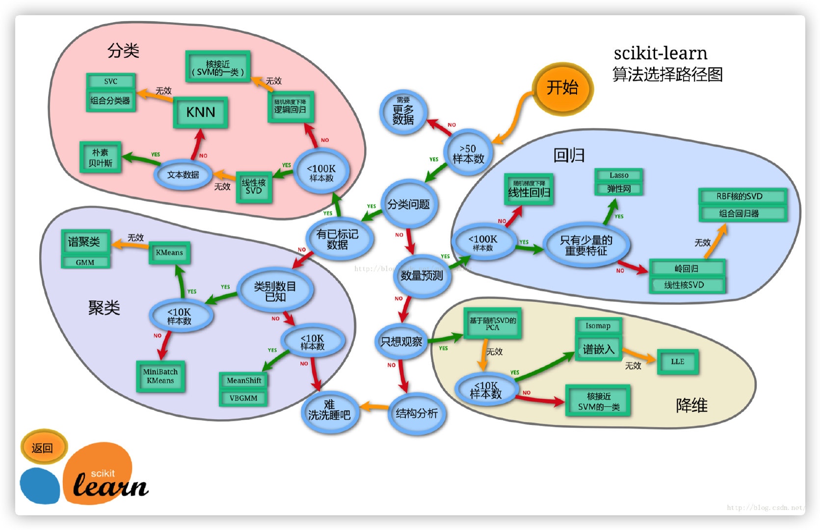sklearn model algorithm selection path diagram

#使用一个机器学习最常用的一个库（sklearn）来完成我们的模型的搭建
#任务一：划分训练集和测试集
'''
将数据集分为自变量和因变量
按比例切割训练集和测试集(一般测试集的比例有30%、25%、20%、15%和10%)
使用分层抽样
设置随机种子以便结果能复现
'''
from sklearn.model_selection import train_test_split
# 一般先取出X和y后再切割，有些情况会使用到未切割的，这时候X和y就可以用,x是清洗好的数据，y是我们要预测的存活数据'Survived'
X = data
y = train['Survived']
# 对数据集进行切割
X_train, X_test, y_train, y_test = train_test_split(X, y, stratify=y, random_state=0)
# 查看数据形状
X_train.shape, X_test.shape

#任务二：模型建立
'''
创建基于线性模型的分类模型（逻辑回归）
创建基于树的分类模型（决策树、随机森林）
分别使用这些模型进行训练，分别的到训练集和测试集的得分
查看模型的参数，并更改参数值，观察模型变化
'''
from sklearn.linear_model import LogisticRegression
from sklearn.ensemble import RandomForestClassifier
# 默认参数逻辑回归模型
lr = LogisticRegression()
lr.fit(X_train, y_train)
# 查看训练集和测试集score值
print("Training set score: {:.2f}".format(lr.score(X_train, y_train)))
print("Testing set score: {:.2f}".format(lr.score(X_test, y_test)))
# 调整参数后的逻辑回归模型
lr2 = LogisticRegression(C=100)
lr2.fit(X_train, y_train)
print("Training set score: {:.2f}".format(lr2.score(X_train, y_train)))
print("Testing set score: {:.2f}".format(lr2.score(X_test, y_test)))
# 默认参数的随机森林分类模型
rfc = RandomForestClassifier()
rfc.fit(X_train, y_train)
print("Training set score: {:.2f}".format(rfc.score(X_train, y_train)))
print("Testing set score: {:.2f}".format(rfc.score(X_test, y_test)))
# 调整参数后的随机森林分类模型
rfc2 = RandomForestClassifier(n_estimators=100, max_depth=5)
rfc2.fit(X_train, y_train)
print("Training set score: {:.2f}".format(rfc2.score(X_train, y_train)))
print("Testing set score: {:.2f}".format(rfc2.score(X_test, y_test)))

#任务三：输出模型预测结果
'''
输出模型预测分类标签
输出不同分类标签的预测概率
'''
# 预测标签
pred = lr.predict(X_train)
# 看到0和1的数组
pred[:10]
# 预测标签概率
pred_proba = lr.predict_proba(X_train)
pred_proba[:10]


#模型搭建和评估-评估模型好不好用
'''
模型评估是为了知道模型的泛化能力。
交叉验证（cross-validation）是一种评估泛化性能的统计学方法，它比单次划分训练集和测试集的方法更加稳定、全面。
在交叉验证中，数据被多次划分，并且需要训练多个模型。
最常用的交叉验证是 k 折交叉验证（k-fold cross-validation），其中 k 是由用户指定的数字，通常取 5 或 10。
准确率（precision）度量的是被预测为正例的样本中有多少是真正的正例
召回率（recall）度量的是正类样本中有多少被预测为正类
f-分数是准确率与召回率的调和平均
'''
#加载库
import pandas as pd
import numpy as np
import seaborn as sns
import matplotlib.pyplot as plt
from IPython.display import Image
from sklearn.linear_model import LogisticRegression
from sklearn.ensemble import RandomForestClassifier

plt.rcParams['font.sans-serif'] = ['SimHei']  # 用来正常显示中文标签
plt.rcParams['axes.unicode_minus'] = False  # 用来正常显示负号
plt.rcParams['figure.figsize'] = (10, 6)  # 设置输出图片大小

#加载数据，切分测试集和训练集
from sklearn.model_selection import train_test_split
# 一般先取出X和y后再切割，有些情况会使用到未切割的，这时候X和y就可以用,x是清洗好的数据，y是我们要预测的存活数据'Survived'
data = pd.read_csv('clear_data.csv')
train = pd.read_csv('train.csv')
X = data
y = train['Survived']
# 对数据集进行切割
X_train, X_test, y_train, y_test = train_test_split(X, y, stratify=y, random_state=0)
# 默认参数逻辑回归模型
lr = LogisticRegression()
lr.fit(X_train, y_train)

#任务一：交叉验证
'''
用10折交叉验证来评估之前的逻辑回归模型
计算交叉验证精度的平均值
'''
#交叉验证在sklearn中的模块为sklearn.model_selection
from sklearn.model_selection import cross_val_score

lr = LogisticRegression(C=100)
scores = cross_val_score(lr, X_train, y_train, cv=10)

# k折交叉验证分数
scores

#平均交叉验证
print("Average cross-validation score: {:.2f}".format(scores.mean()))
'''
思考：k折越多的情况下会带来什么样的影响？
一般而言，k折越多，评估结果的稳定性和保真性越高，不过整个计算复杂度越高。一种特殊的情况是k=m，m为数据集样本个数，这种特例称为留一法，结果往往比较准确
'''


#任务二：混淆矩阵
'''
计算二分类问题的混淆矩阵
计算精确率、召回率以及f-分数
问题：什么是二分类问题的混淆矩阵，理解这个概念，知道它主要是运算到什么任务中的
答：二分类问题的混淆矩阵是一个2维方阵，它主要用于评估二分类问题的好坏，它主要运用于二分类任务中。实际上，多分类问题依然可以转换为二分类问题进行处理。
'''
from sklearn.metrics import confusion_matrix
from sklearn.metrics import classification_report

# 训练模型
lr = LogisticRegression(C=100)
lr.fit(X_train, y_train)

# 模型预测结果
pred = lr.predict(X_train)

# 混淆矩阵
print(confusion_matrix(y_train, pred))

# 精确率、召回率以及f1-score
print(classification_report(y_train, pred))

#任务三：ROC曲线
#绘制ROC曲线
'''
什么是ROC曲线，ROC曲线的存在是为了解决什么问题
ROC的全称是Receiver Operating Characteristic Curve，中文名字叫“受试者工作特征曲线”，其主要的分析方法就是画这条特征曲线，ROC曲线的存在主要用于衡量模型的泛化性能，即分类效果的好坏。
'''
#ROC曲线在sklearn中的模块为sklearn.metrics
#ROC曲线下面所包围的面积越大越好
from sklearn.metrics import roc_curve

fpr, tpr, thresholds = roc_curve(y_test, lr.decision_function(X_test))
plt.plot(fpr, tpr, label="ROC Curve")
plt.xlabel("FPR")
plt.ylabel("TPR (recall)")
# 找到最接近于0的阈值
close_zero = np.argmin(np.abs(thresholds))
plt.plot(fpr[close_zero], tpr[close_zero], 'o', markersize=10, label="threshold zero", fillstyle="none", c='k', mew=2)
plt.legend(loc=4)

'''
思考：对于多分类问题如何绘制ROC曲线?
经典的ROC曲线适用于对二分类问题进行模型评估，通常将它推广到多分类问题的方式有两种：对于每种类别，分别计算其将所有样本点的预测概率作为阈值所得到的TPR和FPR值(是这种类别为正，其他类别为负)，最后将每个取定的阈值下，对应所有类别的TPR值和FPR值分别求平均，得到最终对应这个阈值的TPR和FPR值。
首先，对于一个测试样本：1）标签只由0和1组成，1的位置表明了它的类别（可对应二分类问题中的“正”），0就表示其他类别（“负”）；2）要是分类器对该测试样本分类正确，则该样本标签中1对应的位置在概率矩阵P中的值是大于0对应的位置的概率值的。
参考链接https://blog.csdn.net/qq_30992103/article/details/99730059
'''

The content of this issue mainly learns to use some libraries in Python, especially Pandas and numpy for data analysis, data cleaning, feature value selection, data visualization, data modeling and evaluation, etc., and can learn the workflow of data processing In the later stage, it is necessary to strengthen the practice of the code and the process of drawing inferences from one instance. Many codes are very general and can be used to process many data sets. It is worth practicing and learning many times.

---

Thank you for watching, if you find it helpful, please like or pay attention!
Blog URL: https://7988888.xyz/

Zhihu website: https://www.zhihu.com/people/braintechnology

Knowledge Planet: https://t.zsxq.com/aeimaqv

The content of this article refers to the above URL. The above content is only for learning and not for other purposes. If there is any infringement, please contact us by leaving a message and delete it!

If you have any questions and suggestions, scan the QR code of the following official account to add communication: