Summary of DeepLab series (v1, v2, v3, v3+)

Semantic Segmentation Challenges

• resolution
  • Problem: Continuous pooling or downsampling operations will cause the resolution of the image to drop significantly, thereby losing the original information, and it is difficult to recover during the upsampling process
  • Ways to reduce loss of resolution:
    • dilated convolution
    • Replace pooling with convolution operation with stride 2
• multi-scale features
  • Sending feature maps of different scales into the network for fusion greatly improves the performance of the entire network
  • However, due to the multi-scale input of the image pyramid, a large number of gradients are saved during calculation, which leads to high hardware requirements.
  • The network is trained at multiple scales, and multi-scale fusion is performed in the test phase. If the network encounters a bottleneck, you can consider introducing multi-scale information to help improve network performance.

1. DeepLab v1——《Semantic Image Segmentation with Deep Convolutional Nets and Fully Connected CRFs》（ICLR 2015，谷歌）

• Title: Semantic Image Segmentation with Deep Convolutional Networks and Fully Connected CRF

• Paper: https://arxiv.org/pdf/1412.7062v4.pdf

• Code: https://bitbucket.org/deeplab/deeplab-public/src/master/ (office)

• Research results and significance:

  • 1. The parameters are reduced year-on-year, so the proportion of memory is reduced and the speed is fast
  • 2. With the introduction of ResNet, the deeper the network, the higher the accuracy
  • 3. Continuous convolution and pooling will inevitably lead to a reduction in resolution, but hole convolution can expand the field of view while ensuring the resolution as much as possible
  • 4. The pioneering work of ASPP

• Summary:

  • Background overview : The last layer of DCNNs is not enough for accurate object segmentation
  • Main contribution : This paper combines deep convolutional neural network and CRF to overcome the localization characteristics of deep network
  • Network Effects : DeepLab v1 exceeds the accuracy level of previous methods and can better locate segmentation boundaries
  • Experimental results : 71.6% IOU was obtained in the PASCAL VOC 2012 data set; the processing speed can reach 8 frames per second on a normal GPU

• introduction

  • DeepLab v1 is a method combining Deep Convolutional Neural Networks (DCNNs) and Probabilistic Graphical Models (DenseCRFs)
    Deep Convolutional Neural Networks (DCNNs)
    • 1. Using the FCN idea, modify the VGG16 network, get the coarse score map and interpolate it to the original image size
    • 2. Use Atrous convolution to get a feature map probability model (DenseCRFs) that is denser and has an unchanged receptive field
    • 3. Use the fully connected CRF to refine the details of the segmentation results obtained from DCNNs.

• Algorithms & Experiments

  • 1. Change the fully connected layer (fc6, fc7, fc8) to a convolutional layer (end-to-end training)
  • 2. Change the step size 2 of the last two pooling layers (pool4, pool5) to 1 (to ensure the resolution of the feature)
  • 3. Set the dilate rate of the last three convolutional layers (conv5_1, conv5_2, conv5_3) to 2, and set the dilate rate of the first fully connected layer to 4 (keep the receptive field)
  • 4. Change the number of channels of the last fully connected layer fc8 from 1000 to 21 (the number of categories is 21)
  • 5. In the first fully connected layer fc6, the number of channels changed from 4096 to 1024, and the size of the convolution kernel changed from 7x7 to 3x3. In subsequent experiments, it was found that when the dilate rate here was 12 (LargeFOV), the effect was the best
    
    .
    
    

• Experimental setup:

  • DeepLab-MSc: Similar to FCN, adding feature fusion
  • DeepLab-7×7: Replace the fully connected convolution kernel with a size of 7×7
  • DeepLab-4×4: Replace the fully connected convolution kernel with a size of 4×4
  • DeepLab-LargeFOV: Replace the fully connected convolution kernel with a size of 3×3 and a hole rate of 12
    

2. DeepLab v2——《DeepLab: Semantic Image Segmentation with Deep Convolutional Nets, Atrous Convolution, and Fully Connected CRFs》（TPAMI 2017，谷歌）

• Title: Learning Semantic Segmentation with Deconvolutional Networks
• Paper: https://arxiv.org/pdf/1606.00915v2.pdf (https://arxiv.org/ftp/arxiv/papers/1612/1612.05360.pdf)
• Code: https://github.com/tensorflow/models/tree/master/research/deeplab
• Summary:
  • Main contribution
    : Make full use of the hole convolution, which can effectively expand the receptive field and incorporate more context information without increasing the amount of parameters ; combine DCNNs and CRF to further optimize the network effect; propose the ASPP module
  • Network effect : ASPP enhances the robustness of the network in multi-category segmentation at multiple scales, uses different sampling ratios and receptive fields to extract input features, and can capture target and context information at multiple scales
  • Experimental results : 79.7% MIOU was obtained in the PASCAL VOC 2012 data set; full experiments were also carried out in other data sets
• introduction
  • 1. For feature maps with too low resolution. The article avoids excessive loss of feature map resolution by modifying the last few pooling operations. By introducing hole convolution, the receptive field is increased without increasing parameters and calculations (basically the same as v1)
  • 2. The targets that need to be segmented have various scales. In response to this problem, the article refers to the idea of ​​spatial pyramid pooling, where different proportions of dilated convolutions are used to construct a "spatial pyramid structure" (Atrous Spatial Pyramid Pooling, ASPP)
  • 3. The segmentation accuracy of the DCNN network for the target boundary is not high. The article introduces a fully-connected Conditional Random Field (CRF) to make the positioning of the segmentation boundary more accurate, thus solving this problem
• Prior Knowledge
  • Atrous convolution:
    
    • Receptive field calculation: $R{F}_{1+1}=R{F}_1+(kerne{l}_{s}ize-1)\times stride$
    • Hole rate corresponds to convolution kernel size: $k_{new}=k_{ori}+(k_{ori}-1)(rate-1)$
  • SPPNet(《Spatial Pyramid Pooling in Deep Convolutional Networks for Visual Recognition》)
    • The original intention of SPPNet is to solve the limitation of CNN on the size of input pictures. Due to the existence of the fully connected layer, the output features of the last convolutional layer connected to it need to be fixed in size, thus requiring the input image size to be fixed as well. The previous practice of SPPNet was to crop or deform the picture (crop/warp). However, one problem with crop/warp is that the information of the image is missing or deformed, which affects the recognition accuracy.
      
      
  • bottom-up&top-down
    - top-down: contextual information is used in the process of pattern recognition (for example: when you see a handwritten text with illegible handwriting, you can use the whole text to help you understand the meaning, Instead of identifying each word individually. Because of the contextual information of the surrounding fonts, the brain can perceive and understand the meaning of the text.)
    - bottom-up: data-driven (for example: a person sees a A flower, all visual information about the flower is transmitted from the retina to the brain through the optic nerve, and the brain analyzes the image to determine that it is a flower. The transmission of these information is unidirectional)
  • ResNet
    • Rate of change: The introduction of residuals removes the main part, thus highlighting small changes
    • The main idea: It is more difficult to use a neural network to fit an identity map like y=x than to use a neural network to fit a 0 map like y=0. Because when fitting y=0, you only need to approach the weight and bias to 0.
• Algorithms & Experiments
  • Network&ASPP
    
    
• experiment settings
  • Loss function: cross entropy + softmax
  • Optimizer: SGD + momentum 0.9
  • batchsize：20
  • Learning rate: 10-3 (every 2000 times, learning rate * 0.1)
    
• experiment analysis
  • LargeFOV: 3×3 convolution + rate=12 (the best result of DeepLab v1)
  • ASPP-S：r = 2, 4, 8, 12
  • ASPP-L：r = 6, 12, 18, 24
    
    
    
    
    

3. DeepLab v3 ——《Rethinking Atrous Convolution for Semantic Image Segmentation》（谷歌）

• Title: Learning Semantic Segmentation with Deconvolutional Networks
• Paper: https://arxiv.org/pdf/1706.05587v3.pdf
• Code: https://github.com/tensorflow/models/tree/master/research/deeplab
• Summary:
  • Main contribution : In order to solve the multi-scale segmentation problem, this paper designs a cascaded or parallel dilated convolution module
    ; expands the ASPP module
  • Network effect : the network can get good results without DenseCRF post-processing
  • Experimental results : Comparable performance to other state-of-the-art models is achieved on the PASCAL VOC 2012 dataset
• Contributed to this article
  • 1. This article re-discusses the use of hole convolution, which allows us to obtain a larger receptive field and obtain multi-scale information under the framework of serial modules and spatial pyramid pooling
  • 2. Improved the ASPP module: composed of dilated convolutions and BN layers with different sampling rates, we try to lay out the modules in a serial or parallel manner
  • 3. Discussed an important issue: use a large sampling rate of 3×3 hole convolution, because the image boundary response cannot capture long-distance information (small targets), it will degenerate into a 1×1 convolution, we recommend image-level Feature fusion into ASPP module
• Prior Knowledge
  • Common feature extraction framework for semantic segmentation
    
• Algorithms & Experiments
  
• experiment settings
  • Deep Learning Framework: TensorFlow
  • Crop size: Crop the picture to 513*513
  • Learning rate strategy: adopt poly strategy, the principle is the same as v2
  • BN layer strategy:
    • When output_stride=16, batchsize=16, and at the same time, the parameter attenuation of BN layer is 0.9997
    • On the augmented dataset, freeze the BN layer parameters after training for 30K with an initial learning rate of 0.007
    • When output_stride=8, batchsize=8, use initial learning rate 0.001 to train 30K

4. DeepLab v3+ ——《Encoder-Decoder with Atrous Separable Convolution for Semantic Image Segmentation》（ECCV 2018， 谷歌）

• Title: Learning Semantic Segmentation with Deconvolutional Networks
• Paper: https://arxiv.org/pdf/1802.02611v3.pdf
• code:
  • https://github.com/tensorflow/models(office,Tensorflow)
  • https://github.com/open-mmlab/mmsegmentation(PyTorch)
• Summary:
  • Background overview: Deep neural networks usually use ASPP modules or codec structures for semantic segmentation
  • Main contribution: Extend DeepLab v3 by adding a simple yet effective decoder module to optimize segmentation results
  • Network Effects: The network exceeds the accuracy level of previous methods and can better localize segmentation boundaries
  • Experimental results: 89% and 82.1% MIOU were obtained in the PASCAL VOC 2012 dataset and the Cityscapes dataset respectively
• This article contributes:
  • 1. Proposed an encoder-decoder structure, using DeepLab v3 as the encoder, adding a decoder to get a new model (DeepLabv3+)
  • 2. The Xception model is applied to the segmentation task, and the depth separable convolution is widely used in the model
• Prior Knowledge
  • Depthwise separable convolution (Depthwise separable convolution) ( CSDN: Depthwise separable convolution )
    • The input image size is 12×12×3, and the convolution operation is performed with a 5×5×3 convolution kernel, and an output of 8×8×1 is obtained; 256 5×5×3 convolution kernels are used for Convolution operation, will get 8×8×256 output
    • Parameter calculation: 256×5×5×3 = 19200
      
      
    • Depthwise separable convolution = depthwise convolution + pointwise convolution
    • Depth convolution: Each 5×5×1 convolution kernel corresponds to a channel in the input image, and three 8×8×1 outputs are obtained, and the result of 8×8×3 is obtained after splicing
    • Point-by-point convolution: set 256 1×1×3 convolution kernels, perform convolution operations on the output of depth convolution, and finally obtain an output of 8×8×256
    • Parameter calculation:
      • Depth Convolution Parameters = 5×5×3 = 75
      • Pointwise convolution parameters = 256×1×1×3 = 768
      • Total parameters = 75 + 768 = 843 << 19200
        
        
• Algorithms & Experiments
  • Encoder:
    • 1. Using DeepLab v3 as the encoder structure, the ratio of output to input size is 16 (output_stride = 16)
    • 2.ASPP: One 1×1 convolution + three 3×3 convolutions (rate = {6, 12, 18}) + global average pooling
  • decoder:
    • 1. First upsample the result of the encoder by 4 times, then stitch and fuse it with the feature map of the corresponding size in the encoder, then perform 3x3 convolution, and finally upsample by 4 times to get the final result
    • 2. Before fusing low-level information, perform 1x1 convolution first, in order to reduce the number of channels
      
  • DeepLab v3+ has fine-tuned Xception:
    • 1. Deeper Xception structure, the original middle flow iterates 8 times, and iterates 16 times after fine-tuning
    • 2. All max pooling structures are replaced by depthwise separable convolutions with stride=2
    • 3. Each 3x3 depthwise convolution is followed by BN and Relu
      
• experiment settings
  • Deep Learning Framework: TensorFlow
  • Crop size: Crop the picture to 513*513
  • Learning rate strategy: adopt poly strategy, the principle is the same as v2 v3
    

5. Summary of the paper

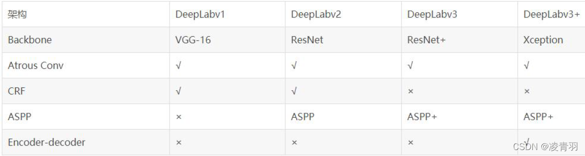
• The development history of DeepLab series:
  • v1: Modify the classic classification network (VGG16), apply hole convolution to the model, try to solve the problem of low resolution and extract multi-scale features, and use CRF for post-processing
  • v2: Design the ASPP module to maximize the performance of dilated convolution, use VGG16 as the main network, try to use ResNet-101 for comparative experiments, and use CRF for post-processing
  • v3: With ResNet as the main network, a serial and a parallel DCNN network are designed, the ASPP module is fine-tuned, and CRF is canceled for post-processing
  • v3+: use ResNet or Xception as the main network, design a new algorithm model combined with the codec structure, use v3 as the encoder structure, design a decoder structure separately, cancel CRF for post-processing