The so-called Martingale strategy is to increase the bet by a multiple of 2 every time you "lose" in a certain gambling market until you win. Assuming that in a fair betting market, the probability of opening big and small is 50%, so at any point in time, the probability of our winning once is 50%, and the probability of winning twice in a row is 25%. The probability of winning three times is 12.5%, the probability of winning four times in a row is 6.25%, and so on. Similarly, the probability of losing streak is the same. Therefore, in trading, many people try the Martingale-style pyramid increase method to trade. So can martingale strategy increase traders' profits?
In this blog, we will focus on martingales and their application to trading strategies through the following topics. Scan the QR code at the bottom of this article to get all the complete source code, CSV data files and Jupyter Notebook files packaged and downloaded.
What is a martingale?
How does a martingale work?
Martingale's conditional expected value
martingale trading strategy
What is an anti-martingale?
Martingale and Anti-Martingale Trading Strategies in Python
"What is a martingale?"
A random variable is an unknown value or a function that takes on a specific value in each possible trial. It can be discrete or continuous. Below we consider discrete random variables to explain martingale.
A martingale is a sequence of random variables M1, M2, M3...Mn, where
E[Mn+1|Mn] = Mn, n -> 0, 1, ..., n+1 (1)
while E[|Mn+1|] < ∞,
Read as the expected value of Mn+1, since the value of Mn is equal to Mn, i.e. the expected value remains the same.
For a random variable, different values x1, x2, x3, the respective probabilities are p1, p2 and p3, the calculation method of the expected value is:
E[M] = x1 * p1 + x2 * p2 + x3 * p3, more simply the expected value is the same as the arithmetic mean.
Note: Martingale is always defined with respect to some information set and some probability measure. If the information set or the probabilities associated with the process change, the process may no longer be a martingale.
"How does a martingale work?"
Consider a simple game where you flip a fair coin and if it comes up heads you win a dollar and if it comes tails you lose a dollar.
In this game, the probability of heads or tails is always half. So, the average win is equal to 1/2(1) + 1/2(-1) = 0, which means you can't systematically make any extra money by playing a number of rounds (although random gains or losses still It is possible).
Thus, the above situation satisfies the martingale property that in any given round, your expected total payoff remains the same regardless of the outcome of previous rounds.
"Conditional Expectations in Martingale"
The expression on the left side of equation (1) in Martingale's definition is called the "conditional expectation". A conditional expected value (also called a conditional mean) is an average calculated after a set of preconditions has occurred.
The conditional expectation of a random variable X with respect to a variable Z is defined as a (new) random variable Y=E(X|Z)
"Martingale Trading Strategy"
The martingale trading strategy is to double your risk or investment size on losing trades. Since your expected long-term return is still the same (loss when prices fall, gains when prices rise), this strategy works by lowering your average entry price by buying points when prices fall. Therefore, even after a series of losing trades, if a profitable trade occurs, it recovers all losses, including the initial trade amount, because its profit is 2^p=∑ 2^p-1+1.
Advantages and disadvantages of the martingale method. One of the advantages is that since the trader doubles the size of the investment after each losing trade, the strategy helps recover losses and generate profits, improving net income. The main downside is that you don't have a stop loss limit as you increase the size of your investment.
Note: In the event of bankruptcy, you may lose your entire capital, or cause capital drawdowns, requiring additional capital, and if the odds do not improve over the long term, you will keep losing.
"What is an Anti-Martingale?"
In the anti-Martingale strategy, the investment size is doubled when the price moves in a profitable direction, and the investment size is cut in half when there is a loss. The idea is to hope that the stock continues to rise in the trend, which is fine in a momentum-driven market.
Advantages and disadvantages of the anti-martingale strategy. The main advantage of the anti-martingale strategy is that it has minimal risk in adverse conditions, because volume does not increase when it loses. Despite its advantages, anti-martingales are not profitable in the event of prolonged losing trades. Therefore, entry signals should be calculated accurately to avoid losses overriding gained profits.
In the next section, we will build martingale and anti-martingale strategies in Python.
"Martingale and Anti-Martingale Trading Strategies in Python"
We used adjusted closing price data for Apple Inc. stock (AAPL) over 6 months. This data is pulled from the Yahoo Finance website and stored in a csv file.
"Read Stock Data"
AAPL's half-year (July-Dec) 2019 adjusted closing price data has been downloaded below:
# Import the libraries , !pip install "library" for first time installing
import numpy as np, pandas as pd
!pip install pyfolio
import pyfolio as pf

import matplotlib.pyplot as plt
%matplotlib inline
plt.style.use('seaborn-darkgrid')
plt.rcParams['figure.figsize'] = (10,7)

import warnings
warnings.filterwarnings("ignore")
# Load AAPL stock csv data and store to a dataframe
df = pd.read_csv("AAPL.csv")
df = df.rename(columns={'Adj_Close': 'price'})
# Convert Date into Datetime format
df['Date'] = pd.to_datetime(df['Date'])
df.fillna(method='ffill', inplace=True)
# Set date as the index of the dataframe
df.set_index('Date',inplace=True)
df.head()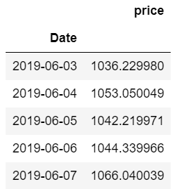
# Create a copy of two dataframes for the trading strategies
df_mg = df.copy()
df_anti_mg = df.copy()
"Simple martingale strategy"
The martingale trading strategy is to double your trade volume on losing trades.
We started with one stock in AAPL and doubled the volume or volume on losing trades. When building the strategy, consider winning trades as a 2% increase from the previous close and losing trades as a decrease of 2% from the previous close.
# Create column for previous price
df_mg['prev_price'] = df_mg['price'].shift(1)

# Generate buy and sell signal for price increase and decrease respectively. And create consolidated 'signal' column by addition of both buy and sell signals
df_mg['long_signal'] = np.where(df_mg['price'] > 1.02*df_mg['prev_price'], 1, 0)
df_mg['short_signal'] = np.where(df_mg['price'] < .98*df_mg['prev_price'], -1, 0)
df_mg['signal'] = df_mg['short_signal'] + df_mg['long_signal']
df_mg.head()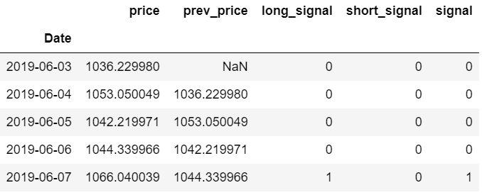
# Initialise 'quantity' column
df_mg['quantity'] = 0

# Start with 1 stock, long position
df_mg['signal'].iloc[0] = 1

# Strategy to double the trade volume or quantity on losing trades
for i in range(df_mg.shape[0]):
  if i == 0:
    df_mg['quantity'].iloc[0] = 1
  else:
    if df_mg['signal'].iloc[i] == 1:
      df_mg['quantity'].iloc[i] = df_mg['quantity'].iloc[i-1]
    if df_mg['signal'].iloc[i] == -1:
      df_mg['quantity'].iloc[i] = df_mg['quantity'].iloc[i-1]*2
    if df_mg['signal'].iloc[i] == 0:
      df_mg['quantity'].iloc[i] = df_mg['quantity'].iloc[i-1]

df_mg.head()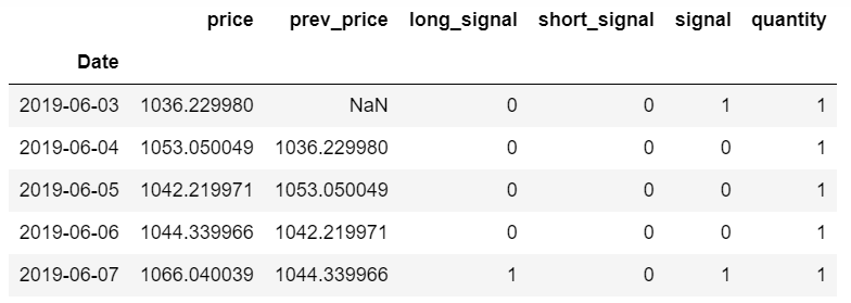
# Calculate returns
df_mg['returns'] = ((df_mg['price'] - df_mg['prev_price'])/ df_mg['price'])*df_mg['quantity']
# Cumulative strategy returns
df_mg['cumulative_returns'] = (df_mg.returns+1).cumprod()
# Plot cumulative returns
plt.figure(figsize=(10,5))
plt.plot(df_mg.cumulative_returns)
plt.grid()
# Define the label for the title of the figure
plt.title('Cumulative Returns for Martingale strategy', fontsize=16)
# Define the labels for x-axis and y-axis
plt.xlabel('Date', fontsize=14)
plt.ylabel('Cumulative Returns', fontsize=14)
# Define the tick size for x-axis and y-axis
plt.xticks(fontsize=12)
plt.yticks(fontsize=12)
plt.show()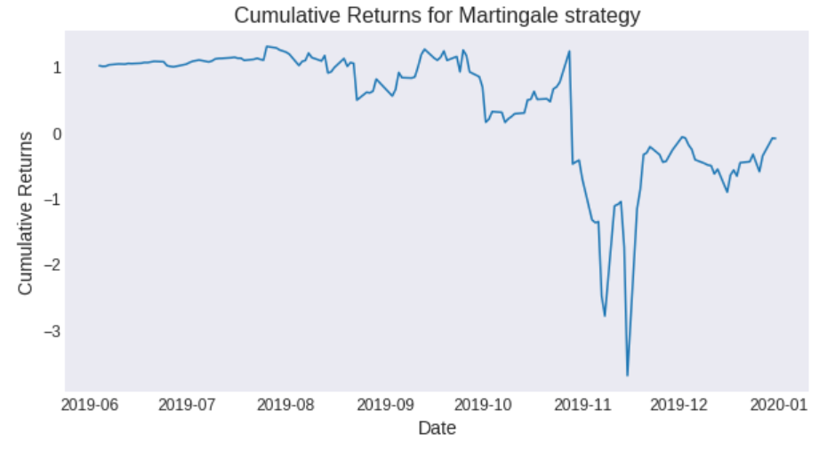
# Plot position
plt.figure(figsize=(10,5))
plt.plot(df_mg.quantity)
plt.grid()

# Define the label for the title of the figure
plt.title('Position sizing', fontsize=16)

# Define the labels for x-axis and y-axis
plt.xlabel('Price', fontsize=14)
plt.ylabel('Quantity', fontsize=14)

# Define the tick size for x-axis and y-axis
plt.xticks(fontsize=12)
plt.yticks(fontsize=12)

plt.show()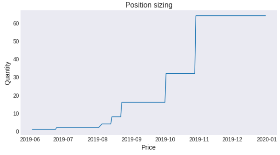
Note: We can notice from the graph above that the volume or volume increases exponentially and so does the cumulative gain. But in this case, we may run out of capital to double the position, leading to bankruptcy.
"Simple Anti-Martingale Strategy"
The anti-martingale strategy is to double the volume on winning trades and halve the volume on losing trades.
Similar to the martingale strategy above, we start with one stock in AAPL and double the volume or amount on winning trades and halve the volume or amount on losing trades. The strategy is built taking into account that winning trades are a 2% increase, while losing trades are a 2% decrease from the previous close.
# This step before deciding trade size is same as the above martingale strategy
# Create column for previous price
df_anti_mg['prev_price'] = df_anti_mg['price'].shift(1)

# Generate buy and sell signal for price increase and decrease respectively. And create consolidated 'signal' column by addition of both buy and sell signals
df_anti_mg['long_signal'] = np.where(df_anti_mg['price'] > 1.02*df_anti_mg['prev_price'], 1, 0)
df_anti_mg['short_signal'] = np.where(df_anti_mg['price'] < .98*df_anti_mg['prev_price'], -1, 0)
df_anti_mg['signal'] = df_anti_mg['short_signal'] + df_anti_mg['long_signal']
df_anti_mg.head()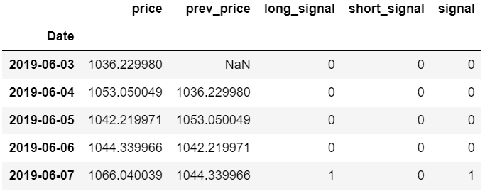
# Intialise 'quantity' column
df_anti_mg['quantity'] = 0

# Start with $10,000 cash long position
cash = 10000
df_anti_mg['signal'].iloc[0] = 1

# Strategy to double the trade volume or quantity on losing trades
for i in range(df_anti_mg.shape[0]):
  if i == 0:
    df_anti_mg['quantity'].iloc[0] = 1
  else:
    if df_anti_mg['signal'].iloc[i] == 1:
      df_anti_mg['quantity'].iloc[i] = df_anti_mg['quantity'].iloc[i-1]*2
    if df_anti_mg['signal'].iloc[i] == -1:
      df_anti_mg['quantity'].iloc[i] = df_anti_mg['quantity'].iloc[i-1]/2
    if df_anti_mg['signal'].iloc[i] == 0:
      df_anti_mg['quantity'].iloc[i] = df_anti_mg['quantity'].iloc[i-1]

df_anti_mg.head()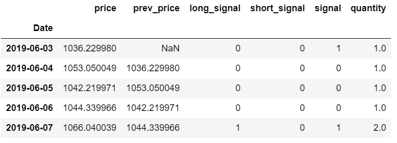
# Calculate returns
df_anti_mg['returns'] = ((df_anti_mg['price'] - df_anti_mg['prev_price'])/ df_anti_mg['prev_price'])*df_anti_mg['quantity']
# Cumulative strategy returns
df_anti_mg['cumulative_returns'] = (df_anti_mg.returns+1).cumprod()
# Plot cumulative returns
plt.figure(figsize=(10,5))
plt.plot(df_anti_mg.cumulative_returns)
plt.grid()
# Define the label for the title of the figure
plt.title('Cumulative Returns for Anti-Martingale strategy', fontsize=16)
# Define the labels for x-axis and y-axis
plt.xlabel('Date', fontsize=14)
plt.ylabel('Cumulative Returns', fontsize=14)
# Define the tick size for x-axis and y-axis
plt.xticks(fontsize=12)
plt.yticks(fontsize=12)
plt.show()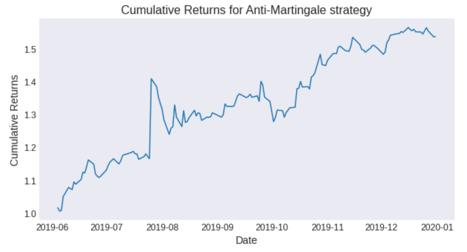
# Plot position
plt.figure(figsize=(10,5))
plt.plot(df_anti_mg.quantity)
plt.grid()

# Define the label for the title of the figure
plt.title('Position sizing', fontsize=16)

# Define the labels for x-axis and y-axis
plt.xlabel('Date', fontsize=14)
plt.ylabel('Quantity', fontsize=14)

# Define the tick size for x-axis and y-axis
plt.xticks(fontsize=12)
plt.yticks(fontsize=12)

plt.show()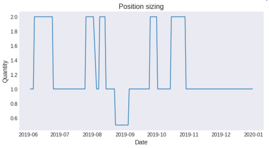
A standard martingale leads to highly variable results in the long run as it can experience exponentially increasing losses. Whereas the reverse martingale distribution of returns is significantly flatter with less variance because it reduces the risk of loss and increases the risk of profit. With this in mind, we see that most successful traders tend to follow the anti-martingale strategy because they are considered less risky to increase the size of their investments during a winning streak than the martingale strategy.
"Summarize"
In this article, we first understand the intuitive meaning of martingale through the concept of conditional expected value. Next, we learned about the types of martingale strategies. Under the martingale trading strategy, the size or volume of the trade is doubled in the losing trade, and the loss is made up by the subsequent profitable trade to generate a profit. In the anti-martingale trading strategy, the trade size or volume is halved on losing trades and doubled on winning trades. We also learned about the market conditions that may be suitable for both strategies. Finally, we implemented martingale and anti-martingale trading strategies in Python.

E N D

Scan the QR code at the bottom of this article to get the source code and data files packaged and downloaded.

↓ ↓ Long press to scan the code to get the complete source code ↓ ↓
