Digital Image Processing--Image Arithmetic Operations

Digital Image Processing – Arithmetic Operations on Images

main content

(1) Perform addition, subtraction, multiplication, and division operations on two different images, and divide them into five sub-windows in the same window to display them separately, and add text titles; (2) Change the grayscale of an image to realize the
image The brightening and darkening of the same window are divided into three sub-windows to display separately, and the text title is marked; the histogram of the three pictures is displayed.

source program

upper code

import cv2
import numpy as np
import matplotlib.pyplot as plt

#灰度变暗函数
def an(mylist):
    for i in range(len(mylist)):
        for each in range(len(mylist[i])):
            #mylist[i][each] = mylist[i][each] - 100
            if mylist[i][each] - 100 < 0:
                mylist[i][each] = 0
            else:
                mylist[i][each] = mylist[i][each] - 100
#灰度变亮函数
def liang(mylist):
    for i in range(len(mylist)):
        for each in range(len(mylist[i])):
            #mylist[i][each] = mylist[i][each] +50
            if mylist[i][each] + 50 > 255:
                mylist[i][each] = 255
            else:
                mylist[i][each] = mylist[i][each] + 50

#读取图片和缩放图片
img_1=cv2.imread('1.png')
img_2=cv2.imread('3.png')
print('img_1_shape:',img_1.shape)
print('img_1:',img_1)
print('**************************')
print('img_2_shape:',img_2.shape)
print('img_2:',img_2)

#两张图片  相加运算
img_add=cv2.add(src1=img_1,src2=img_2)
print('img_add_shape：',img_add.shape)
print('img_add:',img_add)

#两张图片   相减运算
img_sub=cv2.subtract(src1=img_1,src2=img_2)
print('img_sub_shape：',img_sub.shape)
print('img_sub:',img_sub)


#两张图片  相乘运算
img_mul=cv2.multiply(src1=img_1,src2=img_2)
print('img_mul_shape：',img_mul.shape)
print('img_mul:',img_mul)

#两张图片  相除运算
img_div=cv2.divide(src1=img_1,src2=img_2)
print('img_div_shape：',img_div.shape)
print('img_div:',img_div)


print('&&&&&&&&&&&&&&&&&&&&&&&&&&&&&&')
#读取灰度图像2.png
gray = cv2.imread('2.png',cv2.IMREAD_GRAYSCALE)
print(gray.shape)
print('gray',gray)
print('============================')

#绘图
#设置画布标题字体为中文，不设置的话，可能会出现乱码结果
plt.rcParams["font.sans-serif"]=["SimHei"]
plt.rcParams["axes.unicode_minus"]=False

#创建画布，添加标题
plt.gcf().canvas.manager.set_window_title('玫瑰&茉莉花')
plt.gcf().suptitle("玫瑰花&茉莉花")

img_rose = img_1[:,:, ::-1]
img_molly = img_2[:,:,::-1]
img_A = cv2.cvtColor(img_add,cv2.COLOR_BGR2RGB)
img_S = cv2.cvtColor(img_sub,cv2.COLOR_BGR2RGB)
img_M = cv2.cvtColor(img_mul,cv2.COLOR_BGR2RGB)
img_D = cv2.cvtColor(img_div,cv2.COLOR_BGR2RGB)


plt.subplot(231), plt.imshow(img_rose), plt.title("原图-玫瑰花")
plt.subplot(232), plt.imshow(img_molly), plt.title("原图-茉莉花")
plt.subplot(233), plt.imshow(img_A), plt.title("加法")
plt.subplot(234), plt.imshow(img_S), plt.title("减法")
plt.subplot(235), plt.imshow(img_M), plt.title("乘法")
plt.subplot(236), plt.imshow(img_D), plt.title("除法")

plt.figure(2)

#变暗处理
gray_an = gray.copy()
an(gray_an)
print('gray_an_shape',gray_an.shape)
print('gray_an:',gray_an)

#变亮处理
gray_liang = gray.copy()
liang(gray_liang)
print('gray_liang_shape',gray_liang.shape)
print('gray_liang:',gray_liang)



plt.gcf().canvas.manager.set_window_title('灰度图&直方图')
plt.gcf().suptitle('灰度图&直方图')
plt.subplot(231),plt.imshow(gray,cmap='gray'),plt.title('原灰度图')
plt.subplot(232),plt.imshow(gray_an,cmap='gray'),plt.title('变暗')
plt.subplot(233),plt.imshow(gray_liang,cmap='gray'),plt.title('变亮')
plt.subplot(234),plt.hist(gray.ravel(),256),plt.title('原图——直方图')
plt.subplot(235),plt.hist(gray_an.ravel(),256),plt.title('变暗——直方图')
plt.subplot(236),plt.hist(gray_liang.ravel(),256),plt.title('变亮——直方图')


plt.show()

print('total  pixels :',len(gray.ravel()))

achieve results

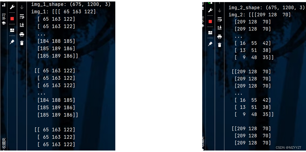
2.1 Read two original images img_1 and img_2 to realize addition, subtraction, multiplication and division operations. Part of the pixel matrix of img_1 and img_2 can be seen from the figure below.

img_1, img_2 pixel matrix

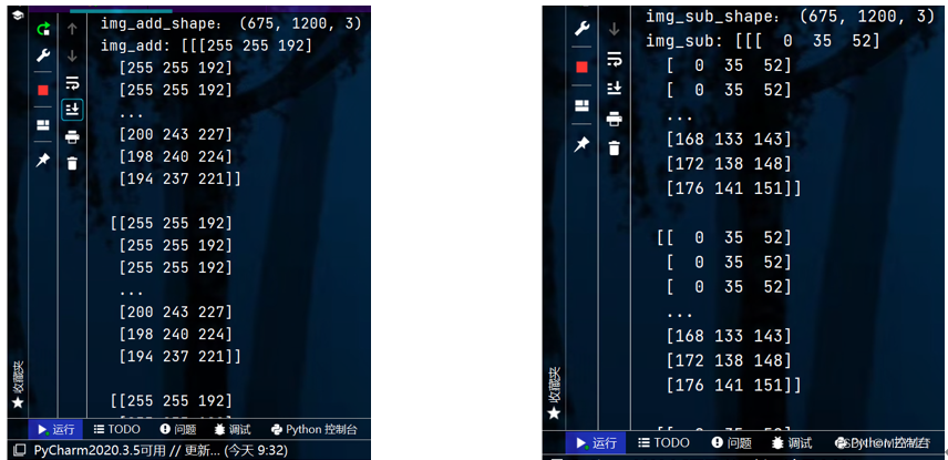
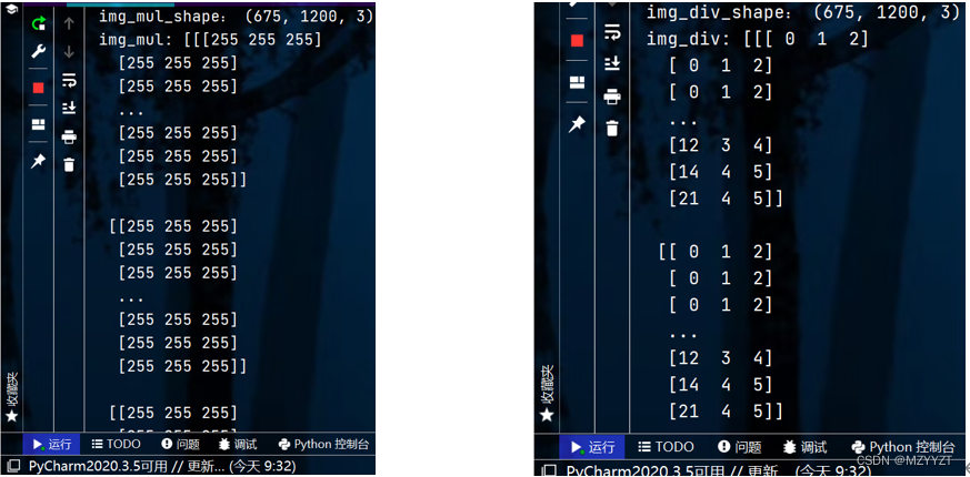
Implement addition, subtraction, multiplication, and division operations on the above img_1 and img_2 and through the following figure, you can find that if the value range (0,255) overflows, the operation of taking 0 or taking 255 will be used.
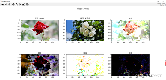
Generate images for the addition, subtraction, multiplication, and


division of the matrices shown above in sequence, as shown in the figure below.

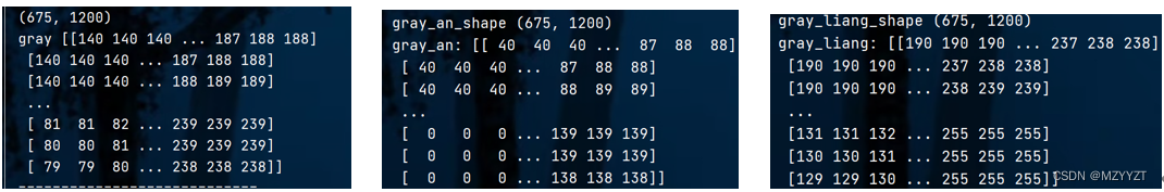
2.2 Grayscale transformation of the image. The resulting pixel matrix after darkening and lightening is shown in the image below.
Original grayscale image, darkened image, brightened image

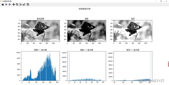
The image generated by the matrix shown in the above figure and its corresponding histogram are shown in the figure below.
Grayscale & histogram

learning records, hope to criticize and correct