Reprinted from : SQL Window Function and Pandas Implementation
Original Author : Data Science Growth Notes
The window function written in the front
provides a simpler data processing method when dealing with complex requirements. It is widely used in actual business and is also a knowledge point that interviewers like to focus on.
What are window functions?
Window function is also called OLAP (Online Analytical Processing) or Analytic Function (Analytic Function). The window refers to the calculation of the set that meets the conditions, and returns the analysis result for each row of data. The format of the window function is as follows:
<window function> OVER (partition by <column name for grouping> order by <column name for sorting> frame_clause)
1. Commonly used window functions
1) 聚合函数:sum()、count()、max()、min()、avg()
2) 排序函数:row_number()、rank()、dense_rank()
3) 分布函数:percent_rank()、cume_dist()
4) 平移函数:lead()、lag()
5) 首尾函数:first_val()、last_val()
2, partition (partition by)
over中partition by类似group by对数据进行分区,此时,窗口函数会对每个分区单独进行分析,如果不指定partition by将会对整体数据进行分析。3. Order by
over中的order by对分区內的数据进行排序,默认为升序,当order by某个字段中有重复值时会对重复值进行求和,然后对所有数据进行累加。4. Window size (frame_clause)
over中的frame_clause指对分区集合指定一个移动窗口,当指定了窗口大小后函数就不会在分区上进行计算,而是基于窗口大小內的数据进行计算。窗口大小的格式如下:rows frame_start
or
rows between frame_start and frame_end
Among them, rows represents the number of offset rows. frame_start indicates the starting position of the window, there are three options:
- UNBOUNDED PRECEDING, which is the default value, means starting from the first line.
- N PRECEDING, means starting from the previous line, if the data in the previous line is missing, it will be 0.
- CURRENT ROW means starting from the current row.
frame_end indicates the end position of the window, there are three options:
- CURRENT ROW is the default value, indicating the end from the current row.
- N FOLLOWING, indicating the end of the Nth line after the current line.
- UNBOUNDED FOLLOWING, indicating that the window ends at the last line of the partition.
The default option in sql is: rows between UNBOUNDED PRECEDING AND CURRENT ROW , indicating that the statistics are from the first row to the current record row.
rows between 1 PRECEDING AND 1 FOLLOWING means that the current row is aggregated with the previous row and the following row, and is mostly used for data statistics in the past N months.
rows between current row and UNBOUNDED FOLLOWING means the current row and all subsequent rows.
Why use window functions
In actual business, we often encounter the need to perform additional statistics on the data results, such as adding a column for the company's overall salary after calculating the salary of employees in each department, or sorting the salary levels of each department, calculating the proportion, etc. At this time, if you do not use the window function, you may need to associate the table multiple times. Therefore, using the window function can greatly simplify the code and improve the read and write performance of the code.
How to use window functions
First of all, according to the definition of window functions, we can know that window functions are mainly divided into types such as aggregation, sorting, distribution, translation, and head and tail. The specific application scenarios for each type are as follows:
aggregate function
Aggregation functions can also act as window functions. We often need to aggregate statistics on the data sets under the window, which is also a widely used category of window functions. For example, we need to count the sales of each employee in each department of company A, and count the maximum, minimum, average and count of each department.
sql implementation
select dept, name, salary,
       sum(salary) over(partition by dept) as sum_salary, --各部门员工薪资求和
       avg(salary) over(partition by dept) as avg_salary, --各部门员工薪资求平均
       min(salary) over(partition by dept) as min_salary, --各部门员工薪资求最小
       max(salary) over(partition by dept) as max_salary  --各部门员工薪资求最大值
from data
Python implementation
import numpy as np
import pandas as pd
company=["A","B","C"]
data=pd.DataFrame({
    "dept":[company[x] for x in np.random.randint(0,len(company),8)],
    "name":["a","b","c","d","e","f","g","h"],
    "salary":np.random.randint(10,30,8)
}
)
data['sum_salary'] = data.groupby('dept')['salary'].transform('sum')
data['min_salary'] = data.groupby('dept')['salary'].transform('min')
data['mean_salary'] = data.groupby('dept')['salary'].transform('mean')
data['max_salary'] = data.groupby('dept')['salary'].transform('max')
data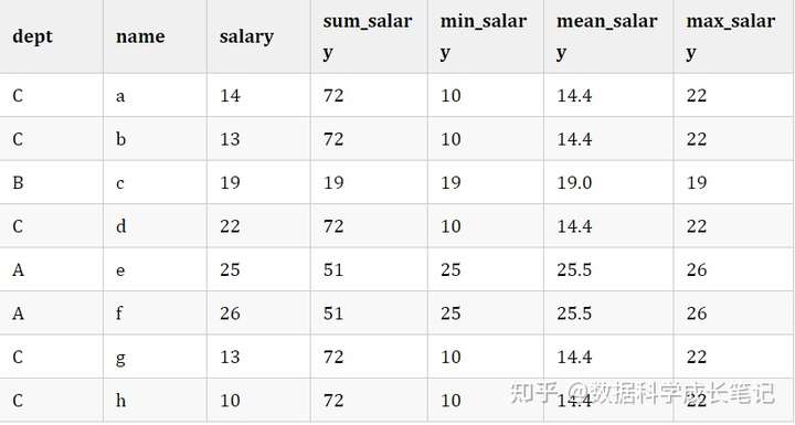
sort function
Sorting functions are often used to rank grouping sets or overall data. For example, we need to sort the salaries of employees in various departments. The sorting functions can be classified as follows according to the sorting method:

1) row_number:对分组內的数据进行"同分不同级"方式排序,不存在序号并列的现象,即使同分时排序也会不同。
2) rank:对分组內的数据进行"同分同级且不紧密"方式排序,当同分时序号相同,其它排序按正常排名进行排序,即1,2,2,4,5。
3) dense_rank:对分组內的数据进行"同分同级且紧密"方式排序,当同分时序号相同,其它排序按下一排名进行排序,即1,2,2,3,4。
sql implementation
select dept, name, salary,
       row_number(salary) over(partition by dept order by salary desc) as row_number, --对各部门员工薪资按同分不同级方式排序
       rank(salary) over(partition by dept order by salary desc) as rank, --对各部门员工薪资按同分同级且紧密方式方式排序
       dense_rank(salary) over(partition by dept order by salary desc) as dense_rank --对各部门员工薪资按同分同级且不紧密方式方式排序
from data
Python implementation
import numpy as np
import pandas as pd
company=["A","B","C"]
data=pd.DataFrame({
    "dept":[company[x] for x in np.random.randint(0,len(company),8)],
    "name":["a","b","c","d","e","f","g","h"],
    "salary":np.random.randint(10,15,8)
}
)
data['row_number'] = data.groupby('dept')['salary'].rank(ascending=False,method='first') #同分不同级
data['rank'] = data.groupby('dept')['salary'].rank(ascending=False,method='min')   #"同分同级且不紧密"
data['dense_rank'] = data.groupby('dept')['salary'].rank(ascending=False,method='dense') #"同分同级且紧密"
data

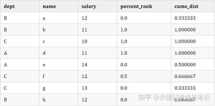
Distribution function
Distribution functions are mainly divided into two categories: percent_rank() and cume_dist().
percent_rank() : refers to calculating the percentage according to the ranking, that is, the ranking is in the interval [0,1], where the first place in the interval is 0, and the last place is 1. Its specific formula is:
percent_rank()=(rank−1)/(rows−1)percent\_rank() = (rank - 1) / (rows - 1) \\
cume_dist() : Refers to the ratio of the number of rows greater than or equal to the current ranking in the interval to the total function in the interval. It is mostly used to judge the proportion of users whose salary and score are higher than the current salary.
sql implementation
select dept, name, salary,
       percent_rank(salary) over(partition by dept order by salary desc) as percent_rank,
       cume_dist(salary) over(partition by dept order by salary desc) as cume_dist
from data
import numpy as np
import pandas as pd
company=["A","B","C"]
data=pd.DataFrame({
    "dept":[company[x] for x in np.random.randint(0,len(company),8)],
    "name":["a","b","c","d","e","f","g","h"],
    "salary":np.random.randint(10,15,8)
}
)
# data.groupby('dept')['salary'].rank(ascending=False,method='first',pct=True)
data['percent_rank'] = (data.groupby('dept')['salary'].rank(ascending=False,method='min')-1) / \
                            (data.groupby('dept')['salary'].transform('count')-1)  #如果分组只有一个记录则数据为na
data['cume_dist'] = data.groupby('dept')['salary'].rank(ascending=False,method='first',pct=True)  #可以结合排序函数的方法使用
data
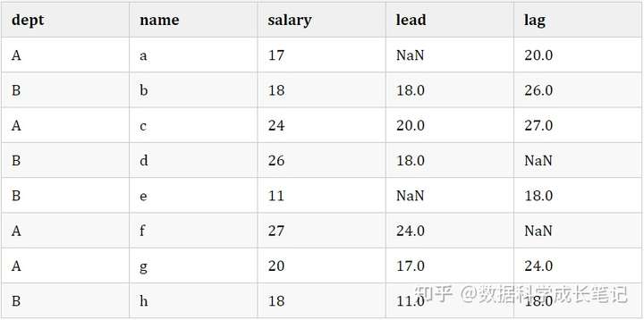
translation function
Distribution functions are mainly divided into two categories: lead (column name, n) and lag (column name, n).
lead(column name, n) : get n rows of data shifted down in the partition.
lag(column name, n) : Get n rows of data shifted up in the partition.
sql implementation
select dept, name, salary,

lead(salary,1) over(partition by dept order by salary desc ) as lead,

lag(salary,1) over(partition by dept order by salary desc) as lag

from data
import numpy as np
import pandas as pd
company=["A","B","C"]
data=pd.DataFrame({
    "dept":[company[x] for x in np.random.randint(0,len(company),8)],
    "name":["a","b","c","d","e","f","g","h"],
    "salary":np.random.randint(10,30,8)
}
)
data['lead'] = data.sort_values(['dept','salary'],ascending=False).groupby('dept')['salary'].shift(-1) # 分区內向下平移一个单位
data['lag'] = data.sort_values(['dept','salary'],ascending=False).groupby('dept')['salary'].shift(1)  # 分区內向上平移一个单位
data
First and last function
Distribution functions are mainly divided into two categories: first_val() and last_val().
first_val() : Get the first row of data in the partition.
last_val() : Get the last row of data in the partition.
sql implementation
select dept, name, salary,

first_val(salary) over(partition by dept order by salary desc ) as first_val,

# 由于窗口函数默认的是第一行至当前行,所以在使用last_val()函数时,会出现分区内最后一行和当前行大小一致的情况,因此我们需要将分区偏移量改为第一行至最后一行。

last_val(salary) over(partition by dept order by salary desc rows between UNBOUNDED PRECEDING and UNBOUNDED FOLLOWING) as last_val

from data
Python implementation
import numpy as np

import pandas as pd

company=[“A”,“B”,“C”]

data=pd.DataFrame({


“dept”:[company[x] for x in np.random.randint(0,len(company),8)],

“name”:[“a”,“b”,“c”,“d”,“e”,“f”,“g”,“h”],

“salary”:np.random.randint(10,30,8)

}

)

data[‘first_val’] = data.groupby(‘dept’)[‘salary’].transform(‘min’)

data[‘last_val’] = data.groupby(‘dept’)[‘salary’].transform(‘max’)

data

Q&A
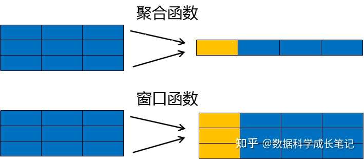
Q1: The difference between aggregate functions and window functions
Difference : Aggregation functions aggregate multiple pieces of data into one row of data, while window functions return a result for each row of data.
Connection : It is all about analyzing a set of data, and window functions can use aggregation functions as functions.
When we need to perform additional statistics on the data results, we often need to use window functions.
Q2: Execution order of SQL
The writing order of SQL is SELECT, FROM, JOIN, ON, WHERE, GROUP BY, HAVING, ORDER BY, LIMIT, and the execution order is shown in the figure below:

Here we need to emphasize the execution order of sql, because in most cases we don’t need to think too much about the execution order of sql, but because the execution order of window functions is located after most fields and only before the field ORDER BY, it is quite It is based on the operation of the window function executed on the basis of executing the temporary table generated by all fields, for example:
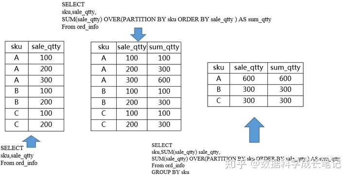
From the above figure, we can see that when the second picture has no GROUP BY and the third picture has GROUP BY, the number of rows of the final data changes from 7 records to 3, because the window function is executed based on the GROUP BY field The calculations are based on the temporary table, so we can easily understand the final results after knowing the execution order of the SQL.