Mathematical programming model summary (with MatLab code)
overview
definition
Mathematical programming is a branch of overall planning, which is used to study: under given conditions ( constraints ), how to find the optimal solution in planning and management work according to a certain row of measurement indicators ( objective function ).
In layman's terms, it is the problem of finding the extreme value of the objective function under certain constraints.
general form
-
min (or max): z = f(x)
-
x: decision variable (generally there are multiple independent variables)
-
f(x): objective function
-
Inequality Constraints, Equality Constraints, Integer Constraints: Constraints
Classification
- linear programming
- nonlinear programming
- integer programming
- 0-1 Planning
linear programming
Both the objective function f(x) and the constraints are linear expressions of the decision variables.
[x fval] = linprog(c, A, b, Aeq, beq, lb,ub, x0)

% X是向量[x1,x2,...xn]' , 即决策变量。(列向量)
% fval 为 function value。
% c是目标函数的系数向量(列向量)
% A是线性不等式约束 Ax<=b 的系数矩阵,b是线性不等式约束 Ax<=b 的常数项(列向量)
% Aeq是线性等式约束 Aeq*x = beq 的系数矩阵,beq是线性等式约束 Aeq*x=beq 的常数项
% lb是X的下限,ub是X的上限。(列向量)
% x0为迭代的初始值(一般不用给)。
Note: The linprog function can only solve the minimum value problem, and the maximum value problem needs to be converted into a minimum value problem by adding a negative sign before the objective function, and the result fval = - fval is enough.
Nonlinear programming
There are nonlinear expressions of the decision variables in the objective function f(x) and constraints.
Note: It is more difficult to solve than linear programming. There is no general algorithm at present. Most algorithms seek the optimal decision variable through a certain search method after the initial decision variable is selected.
[x,fval] = fmincon(@fun,x0,A,b,Aeq,beq,lb,ub,@nonlfun,option)

% x0表示给定的初始值(用行向量或者列向量表示),必须得写
% A b表示线性不等式约束
% Aeq beq 表示线性等式约束
% lb ub 表示上下界约束  lb表示下界 ub表示上界

% @fun表示目标函数
function f = fun1(x)
    f = -x(1)^2-x(2)^2 +x(1)*x(2)+2*x(1)+5*x(2);
end
	% 这里的f实际上就是目标函数,函数的返回值也是f
    % 输入值x实际上就是决策变量,由x1和x2组成的向量

% @nonlfun表示非线性约束的函数
function [c, ceq] = mynonlfun1(x)
    c = [(x(1)-1)^2 - x(2)];     % 默认非线性不等式约束为 ≤ 0
    ceq = [x(1)^2 - x(2)];      % 默认非线性等式约束为 = 0
end

% option 表示求解非线性规划使用的方法
% 使用interior point算法 (内点法)
option = optimoptions('fmincon','Algorithm','interior-point')
% 使用SQP算法 (序列二次规划法)
option = optimoptions('fmincon','Algorithm','sqp')
% 使用active set算法 (有效集法)
option = optimoptions('fmincon','Algorithm','active-set')
% 使用trust region reflective (信赖域反射算法)
option = optimoptions('fmincon','Algorithm','trust-region-reflective')
Integer programming
There are mathematical rules that require variables to take integer values, which are divided into linear integer programming and nonlinear integer programming .
Note: The currently popular algorithms for solving integer programming are often only suitable for linear integer programming.
[x,fval] = intlinprog(c,intcon,A,b,Aeq,beq,lb,ub)

% Matlab线性整数规划求解
% intcon 参数可以指定哪些决策变量是整数(行向量)。
0-1 planning (0-1 programming)
A special case of integer programming, integer variables can only take on the values 0 and 1.
[x,fval] = intlinprog(c,intcon,A,b,Aeq,beq,lb,ub)

% 仍然使用线性整数规划的 intlinprog 函数,只不过在lb和ub上做文章。
% 0-1变量的 lb = 0, ub = 1。
max-min model
Find the most favorable strategy under the most unfavorable conditions.
[x,feval] = fminimax(@Fun,x0,A,b,Aeg,beg,lb,ub,@nonlfun,option)
max(feval)

% 目标函数 Fun 用一个函数向量表示
% 其他变量与非线性规划相同
multi-objective programming model
There are multiple objectives in a planning problem.
Solution: Weighted combination of multi-objective functions turns the problem into a single-objective programming.
[x fval] = linprog(c, A, b, Aeq, beq, lb,ub, x0)

% 仍然使用线性规划的 linprog 函数
% c 中系数乘上了相应权重,并除以某一个常数(做标准化)
Note:
- The weighted combination can only be performed after multiple objective functions are unified into a maximization or minimization problem.
- If the dimensions of the objective functions are not the same, they need to be standardized before weighting. The method of standardization is generally to divide the objective function by a certain constant, which means that a certain value of the objective function can be determined empirically.
- When performing weighted summation on multiple objective functions, the weights need to be given by experts in the problem domain. If there is no special requirement in the actual modeling competition, we can have the same weight.
Sensitivity analysis (for weights)
By changing the values of related variables one by one, the law of the magnitude of the key indicators affected by the changes of these factors is explained.
Example of multi-objective programming + sensitivity analysis

%%  多目标规划
w1 = 0.4;  w2 = 0.6;  % 两个目标函数的权重  x1 = 5  x2 = 2
% w1 = 0.5;  w2 = 0.5;  % 两个目标函数的权重  x1 = 5  x2 = 2
% w1 = 0.3;  w2 = 0.7;  % 两个目标函数的权重  x1 = 1  x2 = 6
c = [w1/30*2+w2/2*0.4 ;w1/30*5+w2/2*0.3];  % 线性规划目标函数的系数
A = [-1 -1];  b = -7; % 不等式约束
lb = [0 0]'; ub = [5 6]'; % 上下界
[x,fval] = linprog(c,A,b,[],[],lb,ub) % 求解线性规划时使用 —— 目标函数和约束条件都是线性的
f1 = 2*x(1)+5*x(2)
f2 = 0.4*x(1) + 0.3*x(2)

%% 敏感性分析
clear;clc
W1 = 0.1:0.001:0.5;  W2 = 1- W1;
n =length(W1);
F1 = zeros(n,1);  F2 = zeros(n,1);   X1 = zeros(n,1);  X2 = zeros(n,1);   FVAL = zeros(n,1);
A = [-1 -1];  b = -7; % 不等式约束
lb = [0 0]; ub = [5 6]; % 上下界
for i = 1:n
    w1 = W1(i);  w2 = W2(i);
    c = [w1/30*2+w2/2*0.4 ;w1/30*5+w2/2*0.3];  % 线性规划目标函数的系数
    [x,fval] = linprog(c,A,b,[],[],lb,ub);
    F1(i) = 2*x(1)+5*x(2);
    F2(i) = 0.4*x(1) + 0.3*x(2);
    X1(i) = x(1);
    X2(i) = x(2);
    FVAL(i) = fval;
end

% 「Matlab」“LaTex字符汇总”讲解:https://blog.csdn.net/Robot_Starscream/article/details/89386748
% 在图上可以加上数据游标,按住Alt加鼠标左键可以设置多个数据游标出来。
figure(1)
plot(W1,F1,W1,F2)
xlabel('f_{1}的权重')
ylabel('f_{1}和f_{2}的取值')
legend('f_{1}','f_{2}')

figure(2)
plot(W1,X1,W1,X2)
xlabel('f_{1}的权重')
ylabel('x_{1}和x_{2}的取值')
legend('x_{1}','x_{2}')

figure(3)
plot(W1,FVAL)  % 看起来是两个直线组合起来的下半部分
xlabel('f_{1}的权重')
ylabel('综合指标的值')
Typical example
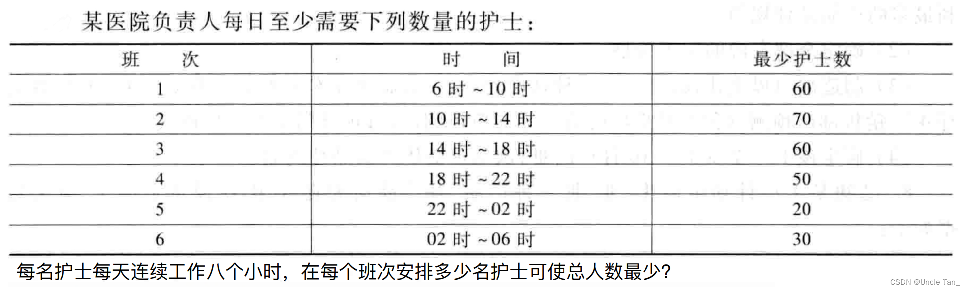
Example 1: Nurse scheduling problem
MatLab code
%% 分析问题为 整数规划 问题
clear;clc
c = ones(6,1);
intcon = 1:6;
A = -[ 1 0 0 0 0 1;
      1 1 0 0 0 0;
      0 1 1 0 0 0;
      0 0 1 1 0 0;
      0 0 0 1 1 0;
      0 0 0 0 1 1 ];
b = -[60; 70; 60; 50; 20; 30];
lb = zeros(6, 1);
[x,fval] = intlinprog(c,intcon,A,b,[],[],lb);
disp('班次安排:');
disp(x');
disp([ '护士总数:',num2str(fval)]);
MatLab output
班次安排:
    60    10    50     0    30     0

护士总数:150
Example 2: Cargo aircraft loading problem

MatLab code
%% 分析问题为 线性规划 问题

% 决策变量:xij为将第i个货物装到第j个舱里的吨数;
% 转化前:x11 x12 x13 x21 x22 …… x42 x43
% 转化后:x1  x2  x3  x4  x5  …… x11 x12
% 二维变量一维化,方便后续处理

% 货舱体积限制的线性不等式约束
clear;clc
format long g   %可以将Matlab的计算结果显示为一般的长数字格式(默认会保留四位小数,或使用科学计数法)
A_v = [ eye(3) * 480 eye(3) * 650 eye(3) * 580 eye(3) * 390]; % eye(n) 表示生成n*n的单位阵
b_v = [ 6800; 8700; 5300];

% 货舱重量限制的线性不等式约束
A_w1 = [ eye(3) eye(3) eye(3) eye(3)];
b_w1 = [ 10; 16; 18];
% 货物重量限制的线性不等式约束
A_w2 = [ ones(1, 3) zeros(1, 9);
         zeros(1, 3) ones(1, 3) zeros(1, 6);
         zeros(1, 6) ones(1, 3) zeros(1, 3);
         zeros(1, 9) ones(1, 3)];
b_w2 = [ 18; 15; 23; 12];
% 汇总线性不等式约束
A = [A_v; A_w1; A_w2];
b = [b_v; b_w1; b_w2];

% 每个货舱装载物比例等式约束
Aeq_1 = repmat([1 0 0], 1, 4) / 10 - repmat([0 1 0], 1, 4) / 16; % 货舱一和货舱二重量成比例
Aeq_2 = repmat([1 0 0], 1, 4) / 10 - repmat([0 0 1], 1, 4) / 8; % 货舱一和货舱三重量成比例
Aeq = [Aeq_1; Aeq_2];
beq = zeros(2, 1)

% 计算飞机利润的系数矩阵
c = -[ones(3, 1) * 3100; ones(3, 1) * 3800; ones(3, 1) * 3500; ones(3, 1) * 2850];
% 每次装运最小值为0
lb = zeros(12, 1);
[x, fval] = linprog(c, A, b, Aeq, beq, lb);
fval = -fval;
% 对 x 做变形转置处理,输出结果
x = reshape(x, 3, 4)';
disp('装运方式:(行为货物,列为货舱)');
disp(x);
disp(['最大飞行利润', num2str(fval)]);
MatLab output
装运方式:(行为货物,列为货舱)
                         0                         0                         0
                        10                         0                         5
                         0          12.9473684210526                         3
                         0          3.05263157894737                         0

最大飞行利润121515.7895
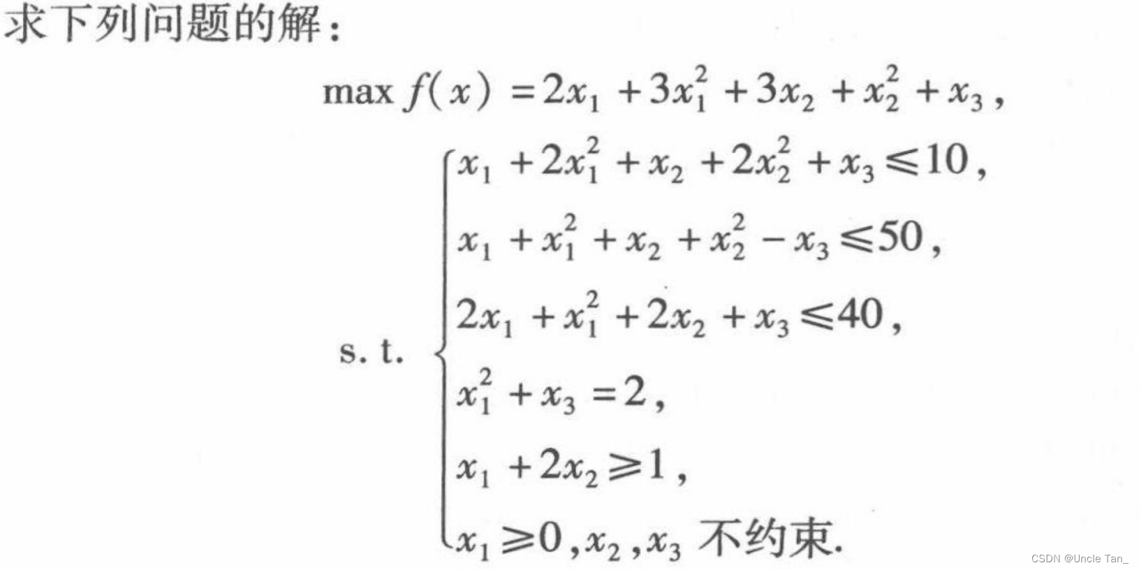
Example 3: Nonlinear programming maximum value problem
MatLab code
%% mainCode部分
clc;clear
format long g   %可以将Matlab的计算结果显示为一般的长数字格式(默认会保留四位小数,或使用科学计数法)

% 给定初始值,此处可以使用蒙特卡洛模拟给定初始值。
x0 = [1 1 1];
% 线性不等式约束
A = [-1 -2 0];
b = 1;
% 决策变量范围约束
lb = [0 -inf -inf];
% 调用函数求解
[x,fval] = fmincon(@fun,x0,A,b,[],[],lb,[],@nonlfun);
fval = -fval
%% fun函数部分
function f = fun(x)
    f = 2 * x(1) + 3 * x(1)^2 + 3 * x(2) + x(2)^2 + x(3);
    f = -f; % 最大值问题转化为最小值问题
end
%% nonlfun函数部分
function [c, ceq] = nonlfun(x)
    % 非线性不等式约束
    c = [x(1) + 2 * x(1)^2 + x(2) + 2 * x(2)^2 + x(3) - 10;
         x(1) + x(1)^2 + x(2) + x(2)^2 - x(3) - 50;
         2 * x(1) + x(1)^2 + 2 * x(2) + x(3) - 40;];
    % 非线性等式约束
    ceq = x(1)^2 + x(3) - 2;
end
MatLab output
x =
          2.33333286682278         0.166667730107356         -3.44444226075484
fval =
          18.0833315976581
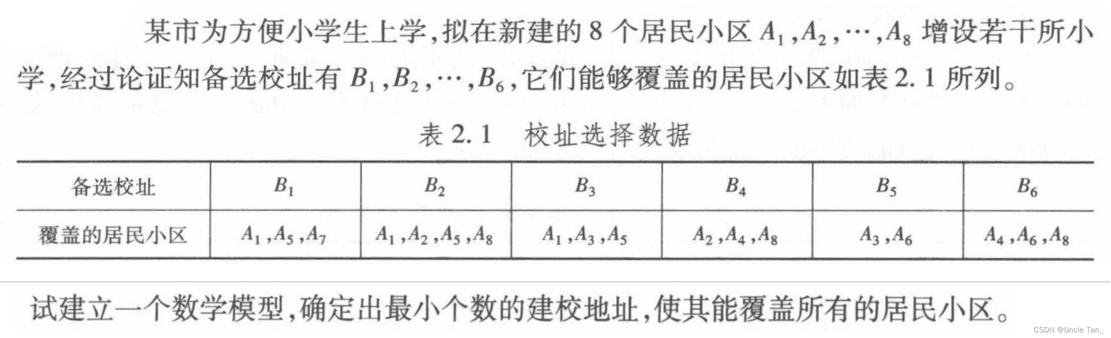
Example 4: Coverage problem
MatLab code
%% 分析问题为 0-1规划 问题
clc;clear
c = ones(6, 1); % 目标函数的系数矩阵
intcon = (1:6); % 整数的位置为1-6
% 保证每一个小区被覆盖的次数 ≥ 1
A = -[1 1 1 0 0 0; % 只有B1 B2 B3 能覆盖A1
      0 1 0 1 0 0;
      0 0 1 0 1 0;
      0 0 0 1 0 1;
      1 1 1 0 0 0;
      0 0 0 0 1 1;
      1 0 0 0 0 0;
      0 1 0 1 0 1;];
b = -ones(8, 1);
% 通过上下限,构建 0-1 分布
lb = zeros(6, 1);
ub = ones(6, 1);
% 调用intlinprog()函数求最优解
[x,fval] = intlinprog(c,intcon,A,b,[],[],lb,ub);
disp('建校方案为:');
for i = 1:6
    if(x(i)) == 1
        disp(['B', num2str(i)]);
    end
end
disp([ '最小建校地址数目:', num2str(fval)]);
MatLab output
建校方案为:
B1
B4
B5
最小建校地址数目:3