Mathematical Modeling - Detailed Explanation of Genetic Algorithm Steps and Programs

Mathematical Modeling - Detailed Explanation of Genetic Algorithm Steps and Programs

---

---

foreword

Genetic algorithm is a principle based on the crossover and mutation of biological chromosome inheritance. It is an algorithm that optimizes and updates the solution set by simulating the natural evolution process. It is a kind of optimization algorithm.

---

1. The basis of genetic algorithm

  The genetic algorithm is based on the principle of biological chromosome inheritance, so it is necessary to understand the basic principles of biology about inheritance. Suppose the population is P(t), and the next generation population is P(t+1)
Inheritance : Excellent individuals in P(t) are passed to the next generation group P(t+1)
Crossover : Individuals in P(t) are randomly matched, and the Each individual exchanges part of the chromosomal
variation with a certain probability : the individual in P(t) changes one or some genes with a certain probability
for evolution : the population gradually adapts to the living environment, and the quality is continuously improved. Biological evolution is carried out in the form of populations.
Fitness : the degree to which a species adapts to the environment in which it lives

1. Encoding and decoding

  Speaking of encoding, the first thing we can think of is the computer binary encoding method. The first thing we do is to change the solution into binary encoding. In the classical genetic algorithm, "chromosome" is used to refer to the individual, which consists of binary strings, as shown in the following figure:

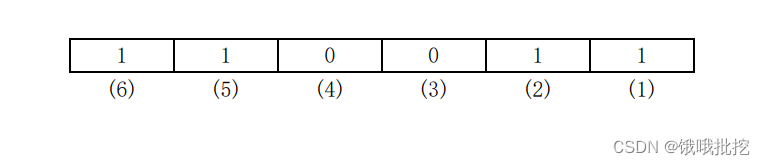
  The above picture can be considered as a chromosome, where 1-0 represents a gene, ( $i$ ) represents the position of the gene.
We first make it clear that the encoding length depends on the range of independent variables (more precisely, the range of decision variables) and search precision, so consider how to encode around them.
  The dimension of the gene represents the information that can be stored, (for example, 000001 represents 1), and the 6-dimensional gene can be converted to decimal to represent$2^{For\; the\; number\; of\; 6}$ , every time one dimension is increased, the number that can be stored is multiplied. But there will be a problem here, the value of the binary expression is multiplied, and sometimes it will not be so coincidental that it will be$2^n$ .
  First, we can determine the range of the independent variable (more accurately, it should be the range of the decision variable) such as (2, 7), assuming that the precision we need is 0.01, then there will be a total of 500 values, and it is greater than 500 and the most A value close to 500 is$2^9$ , 9-digit binary can represent 512-1=511 numbers, we can encode the binary as follows:
$$A_1{A}_2{A}_3\cdots A_9$$
  After encoding, there can be a total of 511 values, which is obviously more than our (2, 7) range of 0.01 accuracy. When encoding, we enlarge 5 to 511, and then reduce it by 511 times when decoding.
When we decode, we can do the following:
$$d=\frac{5}{511}\approx 0.00978$$
First convert the binary code to decimal:
$$A=\sum _{i=1}^n{A}_i{2}^{i-1}$$
and then multiply the decoded decimal number by 0.00978 to get the final result.
$$x=L_X+A\_=L_X+d\sum _{i=1}^n{A}_i{2}^{i-1}$$
  here$L_X$Represents the lower limit of the interval.
  Here you can review the encoding and decoding process. Ordinary binary encoding is the most common encoding method for genetic algorithms. If you learn more in the future, you will have Gray encoding, floating-point encoding, symbol encoding, etc. The first-order coding method will not be expanded here. If you are interested, you can find out by yourself.

2. Fitness function

  The fitness is the degree of adaptability of the species to the living environment, so in the process of the genetic algorithm, the fitness is actually the function corresponding to the solution, which is also called the objective function in the planning model.
①Minimization problem
  makes fitness:
$$F(f(x))=\{\begin{array}{lr}{f}_x-C_{min}& ，f(x)>C_{min}\\ 0& ,other\end{array}$$
  where $C_{min}$The current minimum estimated value②maximization
problem
  makes the fitness:
$$F(f(x))=\{\begin{array}{lr}{C}_{max}-f_x& ，f(x)<C_{max}\\ 0& ,other\end{array}$$
  where $C_{max}$The current maximum estimate
  here introduces two problems of maximization and minimization. In fact, there is also a penalty function problem related to constraints in fitness. In order to solve the constraints of the function, the solution outside the constraints will increase. Function fitness, the greater the distance constraint, the greater the penalty of the penalty function.
②External point method penalty function problem
$$F(x,l)=f(x)+\lambda P(x)$$
$P(x$)的定义一般如下:
$$P\left(x\right)=\sum _{i=1}^{m}p\left(g_i\left(x\right)\right)+\sum _{j=1}^{l}Phi\left(h_j\left(x\right)\right)$$
  whereψ$\psi \left(g_i\right(x\left)\right)$ is a function of inequality constraints, when$When\; x$ is within the inequality constraints,$\psi \left(g_i\right(x\left)\right)$ is zero, when the constraints are not met,$\psi \left(g_i\right(x\left)\right)$ is greater than zero; similarly$Phi\left(h_j\left(x\right)\right)$ is a function with respect to equality constraints. That is, when point$x$ is in the feasible region,$F=f$ , outside the feasible region, F is getting bigger and bigger.
$\psi and\Phi$ are generally defined as follows:
$$p={\left[\max \left(0,-gi\left(x\right)\right)\right]}^a,Phi=|h_j\left(x\right){|}^b$$
In general, take a=b=2
and combine the above formulas to get
$$F\left(x,l\right)=f\left(x\right)+l\left\{\sum _{i=1}^m\max {\left(0,gi\left(x\right)\right)}^2+|h_i\left(x\right){|}^2\right\}$$
  $\lambda$ is a penalty factor, which is a monotonically increasing sequence of positive values,$l^{(k+1)}=e{l}^k$ , experience shows that when e takes [5,10],$l^{(1)}=1$ is relatively satisfactory.

3. Cross

  The DNA at the same position of two chromosomes is cut off, and the two strings before and after are crossed and combined to form two new chromosomes, which is also called genetic recombination or hybridization. Let us use the following example to illustrate, as shown in the figure below:

  The above are the two parent chromosomes. They select a segment of the same position to cross and exchange to get two brand new offspring, as shown in the figure below

  The above is a crossover method, and there are many strange crossover methods. I will not give examples here, but the essence is to intercept a chromosome fragment and perform cross-exchange with other chromosome fragments. Interested students can take a look. Other crossover methods, links are attached below.
https://blog.csdn.net/u012750702/article/details/54563515

4. Variation

  Mutation is much simpler, as long as the code after the crossover is randomly selected to change from 0 to 1 or from 1 to 0. There are also other methods of mutation. The mutation method is to randomly select a few gene positions on the parent chromosome and rearrange them, leaving the other positions unchanged.
  The difference between mutation and crossover is that crossover is two individuals, while mutation is itself. The method of mutation is also strange, and those who are interested can learn about it, and the link is attached below.
https://blog.csdn.net/u011001084/article/details/49450051

5. Choose

  On the basis of evaluating the fitness of the individual, the optimized individual is directly inherited to the next generation through the selection operation, or a new individual is generated through paired crossover and then passed on to the next generation. Suppose the group size is m, the fitness of individual i is Fi, then the probability Pis of individual i being selected is
$$P_{is}=\frac{F_i}{\sum _{i=1}^m{F}_i}$$

2. Principle steps of genetic algorithm

1. Initialization parameters

  After generating the initial solution set, firstly, according to the selection rate, such as selecting a certain proportion of individuals for crossover and mutation process

2. Encoding and decoding

  After the decimal number is converted into a binary number, it is composed of multiple 0s and 1s, which looks more like a chromosome. The crossover process is the cross-exchange of 0 and 1 in the first section of the area, and the mutation is a direct probabilistic 0-1 change. , get the new independent variable and then substitute it into the function to calculate the solution.

3. Select offspring

  After the 90% individuals get the new offspring solution sets, they are arranged from best to worst, and the original parent solution sets are arranged from column to best, and the first 90% of the solutions are directly replaced with the new self-contained solution sets ( A simple understanding is to continuously re-pass the worst 90% solution set through the crossover and mutation process to obtain a new solution set, which may produce a better solution set)

  Therefore, special attention should be paid to the fact that the selection rate (also called generation gap) cannot be set to 100%. Although there is an optimal value record in each cycle, the optimal value can be obtained faster, but it violates the principle of the algorithm, and the algorithm will The approximation becomes a Monte Carlo simulation.

3. Programming and code

The matlab code is as follows:

%遗传算法只能借鉴，因为题目要解决的题不一样，只能借鉴框架,本文代码借鉴了网上的代码
%有疑问可以私聊作者，QQ：2892053776
%先画出大概图像，方便我们后续比较
clc,clear
%遗传算法求解
%matlab是内嵌由遗传工具箱的（不懂的可以百度matlab遗传工具箱）‘
opt_minmax=1;     %目标优化类型：1最大化、-1最小化
num_ppu=50;        %种群规模：个体个数
num_gen=100;       %最大遗传代数
len_ch=9;          %基因长度(二进制位数)
gap=0.9;           %代沟
ub=-1.5;           %变量取值下限
up=3.5;            %变量取值上限
k_gen=0;           %初始化遗传次数
cd_gray=0;         %是否选择格雷编码方式：1是0否
sc_log=0;          %是否选择对数标度：1是0否
trace=zeros(num_gen,2);   %遗传迭代性能跟踪器，生成60行2列0矩阵
chrom=crtbp(num_ppu,len_ch);  %初始化生成种群，生成一个50*20的矩阵，矩阵元素是0-1随机数
%这里没办法运行的可以百度一下安装gatbx遗传包
fieldd=[len_ch;ub;up;1-cd_gray;sc_log;0;0];   %区域描述器
x=bs2rv(chrom,fieldd);            %翻译初始化种群为10进制
fun_v=fun_sigv(x);   %计算目标函数值
tx=ub:.01:up;
plot(tx,fun_sigv(tx))
xlabel('x')
ylabel('y')
title('一元函数优化结果')
hold on
while k_gen<num_gen
    fit_v=ranking(-opt_minmax*fun_v);        %计算目标函数的适应度，适应度应该是越小越好
    %ranking 函数是将适应度压缩在0到2之间，染色体的选择过程比较精巧，使用轮盘赌来对染色体
    %进行选择，而轮盘赌的第一步就是将个体的适应度值取倒数，以便轮盘赌对染色体进行选择。之前我们要取适
    %应度值最小的染色体，但是一旦适应度取了倒数，所有的操作就是相反的了，即轮盘赌取适应度倒数的最大值。
    selchrom=select('rws',chrom,fit_v,gap);  %使用轮盘度方式选择需要交叉变异的个体
    selchrom=recombin('xovsp',selchrom);     %交叉
    selchrom=mut(selchrom);                  %变异
    x=bs2rv(selchrom,fieldd);                %子代个体翻译
    fun_v_sel=fun_sigv(x);                  %计算子代个体对应目标函数值   
    [chrom,fun_v]=reins(chrom,selchrom,1,1,opt_minmax*fun_v,opt_minmax*fun_v_sel);  %根据目标函数值将子代个体插入新种群    
    [f,id]=max(fun_v);                    %寻找当前种群最优解
     x=bs2rv(chrom,fieldd);            %翻译初始化种群为10进制
     f=f*opt_minmax;
     fun_v=fun_v*opt_minmax;
    k_gen=k_gen+1;%记录遗传次数
    trace(k_gen,1)=f;
    trace(k_gen,2)=mean(fun_v);
end
plot(x(id),f,'r*')
figure
plot(trace(:,1),'r-*')
hold on
plot(trace(:,2),'b-o')
legend('各子代种群最优解','各子代种群平均值')
xlabel('迭代次数')
ylabel('目标函数优化情况')
title('一元函数优化过程')

function y=fun_sigv(x)
y=x.*cos(5*pi*x)+2.*x.^2+3.5;

---

Summarize

  The genetic algorithm itself is an optimization algorithm, and it can also be used to solve the traveling salesman problem. Moreover, the genetic algorithm depends on the face. Sometimes even if the number of iterations and the population density are increased, the ideal solution may not be found, and sometimes the result may be obtained in one go.
  In the actual process operation, the problems are ever-changing, and the objective function is also ever-changing, which determines that the objective function, crossover, and mutation processes are relatively complex and changeable, and need to be flexibly changed according to needs.
Advantage
1: The optimization result has nothing to do with the initial conditions.
2: The search starts from the group, which has potential parallelism and can perform simultaneous comparison of multiple individuals.
3: The search is inspired by the evaluation function, and the process is simple.
4: It is scalable and easy to combine with other algorithms. (Genetic simulated annealing algorithm)
Disadvantage
1: The convergence speed is slow, and there is no mathematical proof that it will converge when n approaches infinity.
2: Poor local search ability.
3: There are many control variables.
4: No definitive termination criteria.