12.1.3 Simple code implementation of XGBoost algorithm
The XGBoost model can be used for both classification analysis and regression analysis. The corresponding models are XGBoost classification model (XGBClassifier) and XGBoost regression model (XGBRegressor).
The installation method of the XGBoost model can be the PIP installation method. Take the Windows operating system as an example, the Win+R shortcut key calls out the run box. After entering cmd, enter the code in the pop-up interface and press Enter to run: pip install
xgboost
# 如果是在Jupyter Notebook编辑器中,则可输入如下内容,然后运行该代码块即可(需取消注释):
# !pip install xgboost
1. Classification model
# XGBoost分类模型的引入方式:
from xgboost import XGBClassifier
# 在Jupyter Notebook编辑器中,在引入该库后,可以通过如下代码获取官方讲解内容(需取消注释):
# XGBClassifier?
import numpy as np
np.array([[1, 2], [3, 4], [5, 6], [7, 8], [9, 10]])
array([[ 1,  2],
       [ 3,  4],
       [ 5,  6],
       [ 7,  8],
       [ 9, 10]])
# XGBoost分类模型简单代码演示如下所示:
from xgboost import XGBClassifier
import numpy as np

X = np.array([[1, 2], [3, 4], [5, 6], [7, 8], [9, 10]])  # 2020年升级后必须是numpy或者DataFrame格式
y = [0, 0, 0, 1, 1]

model = XGBClassifier()
model.fit(X, y)

print(model.predict(np.array([[5, 5]])))
[0]
Among them, X is a feature variable, which has 2 features in total; y is the target variable; the fourth line of code uses data of array array type for demonstration, because the feature variables of the XGBoost classification model do not support direct input of list type data, and can be passed in The data in the array format or the data in the DataFrame two-dimensional table format; the seventh line introduces the model; the eighth line trains the model through the fit() function; the last line predicts through the predict() function.
2. Regression model
# XGBoost回归模型的引入方式:
from xgboost import XGBRegressor
# 在Jupyter Notebook编辑器中,在引入该库后,可以通过如下代码获取官方讲解内容(需取消注释):
# XGBRegressor?
# XGBoost回归模型简单代码演示如下所示:
from xgboost import XGBRegressor
import numpy as np

X = np.array([[1, 2], [3, 4], [5, 6], [7, 8], [9, 10]])
y = [1, 2, 3, 4, 5]

model = XGBRegressor()
model.fit(X, y)

print(model.predict(np.array([[5, 5]])))
[3.0000014]
Among them, X is a feature variable, which has 2 features; y is the target variable; the fifth line introduces the model; the sixth line trains the model through the fit() function; the last line predicts through the predict() function.
12.2 XGBoost Algorithm Case 1 - Financial Anti-fraud Model
12.2.1 Case background
Credit card fraud generally occurs when the cardholder's information is stolen by criminals and then the card is copied for consumption or the credit card is activated for consumption after being falsely claimed by others. Once credit card fraud occurs, both the cardholder and the bank will suffer certain economic losses. Therefore, it is particularly important for banks to build a financial anti-fraud model through big data.
12.2.2 Model Construction
1. Read data
import pandas as pd
df = pd.read_excel('信用卡交易数据.xlsx')
df.head()
| Change equipment times | Number of payment failures | Change IP times | Number of IP country changes | Amount of the transaction | Fraud Label | |
|---|---|---|---|---|---|---|
| 0 | 0 | 11 | 3 | 5 | 28836 | 1 |
| 1 | 5 | 6 | 1 | 4 | 21966 | 1 |
| 2 | 6 | 2 | 0 | 0 | 18199 | 1 |
| 3 | 5 | 8 | 2 | 2 | 24803 | 1 |
| 4 | 7 | 10 | 5 | 0 | 26277 | 1 |
2. Extract feature variables and target variables
# 通过如下代码将特征变量和目标变量单独提取出来,代码如下:
X = df.drop(columns='欺诈标签')
y = df['欺诈标签']
3. Divide training set and test set
# 提取完特征变量后,通过如下代码将数据拆分为训练集及测试集:
from sklearn.model_selection import train_test_split
X_train, X_test, y_train, y_test = train_test_split(X, y, test_size=0.2, random_state=123)
4. Model training and construction
# 划分为训练集和测试集之后,就可以引入XGBoost分类器进行模型训练了,代码如下:
from xgboost import XGBClassifier
clf = XGBClassifier(n_estimators=100, learning_rate=0.05)
clf.fit(X_train, y_train)
XGBClassifier(base_score=None, booster=None, callbacks=None,colsample_bylevel=None, colsample_bynode=None, colsample_bytree=None, early_stopping_rounds=None, enable_categorical=False, eval_metric=None, feature_types=None, gamma=None, gpu_id=None, grow_policy=None, importance_type=None, interaction_constraints=None, learning_rate=0.05, max_bin=None, max_cat_threshold=None, max_cat_to_onehot=None, max_delta_step=None, max_depth=None, max_leaves=None, min_child_weight=None, missing=nan, monotone_constraints=None, n_estimators=100, n_jobs=None, num_parallel_tree=None, predictor=None, random_state=None, ...)</pre><b>In a Jupyter environment, please rerun this cell to show the HTML representation or trust the notebook. <br />On GitHub, the HTML representation is unable to render, please try loading this page with nbviewer.org.</b></div><div class="sk-container" hidden><div class="sk-item"><div class="sk-estimator sk-toggleable"><input class="sk-toggleable__control sk-hidden--visually" id="sk-estimator-id-1" type="checkbox" checked><label for="sk-estimator-id-1" class="sk-toggleable__label sk-toggleable__label-arrow">XGBClassifier</label><div class="sk-toggleable__content"><pre>XGBClassifier(base_score=None, booster=None, callbacks=None, colsample_bylevel=None, colsample_bynode=None, colsample_bytree=None, early_stopping_rounds=None, enable_categorical=False, eval_metric=None, feature_types=None, gamma=None, gpu_id=None, grow_policy=None, importance_type=None, interaction_constraints=None, learning_rate=0.05, max_bin=None, max_cat_threshold=None, max_cat_to_onehot=None, max_delta_step=None, max_depth=None, max_leaves=None, min_child_weight=None, missing=nan, monotone_constraints=None, n_estimators=100, n_jobs=None, num_parallel_tree=None, predictor=None, random_state=None, ...)</pre></div></div></div></div></div>
12.2.3 Model prediction and evaluation
# 模型搭建完毕后,通过如下代码预测测试集数据:
y_pred = clf.predict(X_test)

y_pred  # 打印预测结果
array([0, 1, 1, 0, 0, 0, 1, 0, 0, 0, 1, 1, 1, 1, 1, 0, 0, 0, 0, 0, 1, 1,
       1, 0, 0, 0, 0, 0, 0, 1, 0, 1, 0, 1, 0, 0, 1, 1, 1, 0, 0, 1, 0, 0,
       0, 0, 1, 0, 0, 0, 1, 0, 0, 0, 1, 1, 0, 1, 0, 0, 0, 0, 1, 0, 1, 0,
       0, 0, 0, 1, 1, 0, 0, 0, 0, 0, 0, 0, 1, 0, 0, 0, 0, 0, 0, 1, 0, 0,
       0, 1, 0, 0, 0, 1, 1, 0, 0, 0, 0, 0, 0, 0, 0, 0, 0, 0, 1, 0, 0, 1,
       0, 0, 1, 0, 1, 0, 0, 0, 1, 0, 0, 0, 0, 0, 0, 1, 0, 0, 1, 1, 0, 0,
       0, 0, 0, 0, 0, 1, 0, 0, 1, 0, 0, 1, 1, 0, 0, 1, 0, 1, 0, 0, 0, 0,
       1, 0, 1, 1, 1, 0, 1, 0, 1, 1, 1, 0, 0, 0, 0, 0, 0, 0, 0, 0, 0, 0,
       0, 1, 0, 0, 0, 1, 0, 0, 1, 0, 0, 1, 0, 0, 1, 0, 0, 0, 0, 0, 1, 0,
       1, 1])
# 通过和之前章节类似的代码,我们可以将预测值和实际值进行对比:
a = pd.DataFrame()  # 创建一个空DataFrame
a['预测值'] = list(y_pred)
a['实际值'] = list(y_test)
a.head()
| Predictive value | actual value | |
|---|---|---|
| 0 | 0 | 1 |
| 1 | 1 | 1 |
| 2 | 1 | 1 |
| 3 | 0 | 0 |
| 4 | 0 | 1 |
# 可以看到此时前五项的预测准确度为60%,如果想看所有测试集数据的预测准确度,可以使用如下代码:
from sklearn.metrics import accuracy_score
score = accuracy_score(y_pred, y_test)
score
0.875
# 我们还可以通过XGBClassifier()自带的score()函数来查看模型预测的准确度评分,代码如下,获得的结果同样是0.875。
clf.score(X_test, y_test)
0.875
# XGBClassifier分类器本质预测的并不是准确的0或1的分类,而是预测其属于某一分类的概率,可以通过predict_proba()函数查看预测属于各个分类的概率,代码如下:
y_pred_proba = clf.predict_proba(X_test)
print(y_pred_proba[0:5])  # 查看前5个预测的概率
[[0.8265032  0.1734968 ]
 [0.02098632 0.9790137 ]
 [0.0084281  0.9915719 ]
 [0.8999369  0.1000631 ]
 [0.8290514  0.17094862]]
# 此时的y_pred_proba是个二维数组,其中第一列为分类为0(也即非欺诈)的概率,第二列为分类为1(也即欺诈)的概率,因此如果想查看欺诈(分类为1)的概率,可采用如下代码:
# y_pred_proba[:,1]  # 分类为1的概率
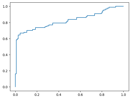
# 下面我们利用4.3节相关代码绘制ROC曲线来评估模型预测的效果:
from sklearn.metrics import roc_curve
fpr, tpr, thres = roc_curve(y_test, y_pred_proba[:,1])
import matplotlib.pyplot as plt
plt.plot(fpr, tpr)
plt.show()

# 通过如下代码求出模型的AUC值:
from sklearn.metrics import roc_auc_score
score = roc_auc_score(y_test, y_pred_proba[:,1])

score
0.8684772657918828
# 我们可以通过查看各个特征的特征重要性(feature importance)来得出信用卡欺诈行为判断中最重要的特征变量:
clf.feature_importances_
array([0.40674362, 0.19018467, 0.04100984, 0.33347663, 0.02858528],
      dtype=float32)
# 通过如下5.2.2节特征重要性相关知识点进行整理,方便结果呈现,代码如下:
features = X.columns  # 获取特征名称
importances = clf.feature_importances_  # 获取特征重要性

# 通过二维表格形式显示
importances_df = pd.DataFrame()
importances_df['特征名称'] = features
importances_df['特征重要性'] = importances
importances_df.sort_values('特征重要性', ascending=False)
| feature name | feature importance | |
|---|---|---|
| 0 | Change equipment times | 0.406744 |
| 3 | Number of IP country changes | 0.333477 |
| 1 | Number of payment failures | 0.190185 |
| 2 | Change IP times | 0.041010 |
| 4 | Amount of the transaction | 0.028585 |
10.2.4 Model parameter tuning
from sklearn.model_selection import GridSearchCV
parameters = {

    'max_depth': [1, 3, 5], 'n_estimators': [50, 100, 150], 'learning_rate': [0.01, 0.05, 0.1, 0.2]}  # 指定模型中参数的范围
clf = XGBClassifier()  # 构建模型
grid_search = GridSearchCV(clf, parameters, scoring='roc_auc', cv=5)
# 下面我们将数据传入网格搜索模型并输出参数最优值:
grid_search.fit(X_train, y_train)  # 传入数据
grid_search.best_params_  # 输出参数的最优值
{'learning_rate': 0.05, 'max_depth': 1, 'n_estimators': 100}
# 下面我们根据新的参数建模,首先重新搭建XGBoost分类器,并将训练集数据传入其中:
clf = XGBClassifier(max_depth=1, n_estimators=100, learning_rate=0.05)
clf.fit(X_train, y_train)
XGBClassifier(base_score=None, booster=None, callbacks=None,colsample_bylevel=None, colsample_bynode=None, colsample_bytree=None, early_stopping_rounds=None, enable_categorical=False, eval_metric=None, feature_types=None, gamma=None, gpu_id=None, grow_policy=None, importance_type=None, interaction_constraints=None, learning_rate=0.05, max_bin=None, max_cat_threshold=None, max_cat_to_onehot=None, max_delta_step=None, max_depth=1, max_leaves=None, min_child_weight=None, missing=nan, monotone_constraints=None, n_estimators=100, n_jobs=None, num_parallel_tree=None, predictor=None, random_state=None, ...)</pre><b>In a Jupyter environment, please rerun this cell to show the HTML representation or trust the notebook. <br />On GitHub, the HTML representation is unable to render, please try loading this page with nbviewer.org.</b></div><div class="sk-container" hidden><div class="sk-item"><div class="sk-estimator sk-toggleable"><input class="sk-toggleable__control sk-hidden--visually" id="sk-estimator-id-2" type="checkbox" checked><label for="sk-estimator-id-2" class="sk-toggleable__label sk-toggleable__label-arrow">XGBClassifier</label><div class="sk-toggleable__content"><pre>XGBClassifier(base_score=None, booster=None, callbacks=None, colsample_bylevel=None, colsample_bynode=None, colsample_bytree=None, early_stopping_rounds=None, enable_categorical=False, eval_metric=None, feature_types=None, gamma=None, gpu_id=None, grow_policy=None, importance_type=None, interaction_constraints=None, learning_rate=0.05, max_bin=None, max_cat_threshold=None, max_cat_to_onehot=None, max_delta_step=None, max_depth=1, max_leaves=None, min_child_weight=None, missing=nan, monotone_constraints=None, n_estimators=100, n_jobs=None, num_parallel_tree=None, predictor=None, random_state=None, ...)</pre></div></div></div></div></div>
# 因为我们是通过ROC曲线的AUC评分作为模型评价准则来进行参数调优的,因此通过如下代码我们来查看新的AUC值:
y_pred_proba = clf.predict_proba(X_test)
from sklearn.metrics import roc_auc_score
score = roc_auc_score(y_test, y_pred_proba[:,1])
print(score)
0.8563218390804598
Print out the obtained AUC score as: 0.856, which is slightly lower than the original 0.866 before parameter adjustment. Some readers may wonder why the result after parameter adjustment is not as good as the result without parameter adjustment. Generally speaking, the parameters The probability of such a situation in tuning is relatively small, and it happens here to explain the reason for this situation.
The reason for this situation is because of cross-validation. Let's briefly review the idea of K-fold cross-validation in section 5.3: it divides the original test data into K parts (here cv=5, that is, 5 parts), and then in this Among the K data, select K-1 as the training data, and the remaining 1 as the test data, train K times, obtain the AUC value under the K ROC curve, and then average the K AUC values to obtain the AUC value The parameter in the case where the mean value of is the maximum is the optimal parameter of the model. Note that the acquisition of the AUC value here is based on the training set data, but only 1/K of the training set data is used as the test set data. The test set data here is not the real test set data y_test, which is why after parameter tuning The result is not as good as the reason for the result of not tuning. In practical applications, it is usually less likely that the results of parameter tuning are not as good as those of no parameter tuning. To some extent, this situation is also due to the small amount of data (such as 1000 pieces of data in this case). Please refer to Section 5.3 for other points of attention about parameter tuning, so I won’t go into details here.
12.3 XGBoost Algorithm Case 2 - Credit Scoring Model
12.3.1 Case Background
In order to reduce the non-performing loan rate, ensure the safety of their own funds, and improve the level of risk control, banks and other financial institutions will build credit scoring models based on customers' credit history data to score customers. According to the customer's credit score, it can estimate the possibility of the customer's repayment on time, and decide whether to grant a loan, the amount and interest rate of the loan.
12.3.2 Multiple Linear Regression Models
1. Read data
import pandas as pd
df = pd.read_excel('信用评分卡模型.xlsx')
df.head()
| monthly income | age | gender | Historical line of credit | Historical defaults | credit score | |
|---|---|---|---|---|---|---|
| 0 | 7783 | 29 | 0 | 32274 | 3 | 73 |
| 1 | 7836 | 40 | 1 | 6681 | 4 | 72 |
| 2 | 6398 | 25 | 0 | 26038 | 2 | 74 |
| 3 | 6483 | 23 | 1 | 24584 | 4 | 65 |
| 4 | 5167 | 23 | 1 | 6710 | 3 | 73 |
2. Extract feature variables and target variables
# 通过如下代码将特征变量和目标变量单独提取出来,代码如下:
X = df.drop(columns='信用评分')
Y = df['信用评分']
3. Model training and construction
# 从Scikit-Learn库中引入LinearRegression()模型进行模型训练,代码如下:
from sklearn.linear_model import LinearRegression
model = LinearRegression()
model.fit(X,Y)
LinearRegression()In a Jupyter environment, please rerun this cell to show the HTML representation or trust the notebook.
On GitHub, the HTML representation is unable to render, please try loading this page with nbviewer.org.
LinearRegression()
# 4.线性回归方程构造
print('各系数为:' + str(model.coef_))
print('常数项系数k0为:' + str(model.intercept_))
各系数为:[ 5.58658996e-04  1.62842002e-01  2.18430276e-01  6.69996665e-05
 -1.51063940e+00]
常数项系数k0为:67.16686603853304
5. Model evaluation
# 利用3.2节模型评估的方法对此多元线性回归模型进行评估,代码如下:
import statsmodels.api as sm
X2 = sm.add_constant(X)
est = sm.OLS(Y, X2).fit()
est.summary()
| Dep. Variable: | credit score | R-squared: | 0.629 |
|---|---|---|---|
| Model: | OLS | Adj. R-squared: | 0.628 |
| Method: | Least Squares | F-statistic: | 337.6 |
| Date: | Mon, 17 Apr 2023 | Prob (F-statistic): | 2.32e-211 |
| Time: | 10:56:44 | Log-Likelihood: | -2969.8 |
| No. Observations: | 1000 | AIC: | 5952. |
| Df Residuals: | 994 | BIC: | 5981. |
| Df Model: | 5 | ||
| Covariance Type: | non-robust |
| coef | std err | t | P>|t| | [0.025 | 0.975] | |
|---|---|---|---|---|---|---|
| const | 67.1669 | 1.121 | 59.906 | 0.000 | 64.967 | 69.367 |
| monthly income | 0.0006 | 8.29e-05 | 6.735 | 0.000 | 0.000 | 0.001 |
| age | 0.1628 | 0.022 | 7.420 | 0.000 | 0.120 | 0.206 |
| gender | 0.2184 | 0.299 | 0.730 | 0.466 | -0.369 | 0.806 |
| Historical line of credit | 6.7e-05 | 7.78e-06 | 8.609 | 0.000 | 5.17e-05 | 8.23e-05 |
| Historical defaults | -1.5106 | 0.140 | -10.811 | 0.000 | -1.785 | -1.236 |
| Omnibus: | 13.180 | Durbin-Watson: | 1.996 |
|---|---|---|---|
| Prob(All): | 0.001 | Jarque-Bera (JB): | 12.534 |
| Skew: | -0.236 | Prob(JB): | 0.00190 |
| Kurtosis: | 2.721 | Cond. No. | 4.27e+05 |
Notes:
[1] Standard Errors assume that the covariance matrix of the errors is correctly specified.
[2] The condition number is large, 4.27e+05. This might indicate that there are
strong multicollinearity or other numerical problems.
It can be seen that the overall R-squared of the model is 0.629, and the Adj. R-Squared is 0.628. The overall fitting effect is average, which may be due to the small amount of data. At the same time, we look at the P value again, and we can find that the P value of most of the characteristic variables is small (less than 0.05), which is indeed significantly related to the target variable: credit score, and the P value of the characteristic variable of gender reaches 0.466, which is related to The target variable has no significant correlation, which is indeed in line with empirical cognition, so in the multiple linear regression model, we can actually discard the characteristic variable of gender.
12.3.3 GBDT Regression Model
# 这里使用第九章讲过的GBDT回归模型同样来做一下回归分析,首先读取1000条信用卡客户的数据并划分特征变量和目标变量,这部分代码和上面线性回归的代码是一样的。
# 1.读取数据
import pandas as pd
df = pd.read_excel('信用评分卡模型.xlsx')
# 2.提取特征变量和目标变量
X = df.drop(columns='信用评分')
y = df['信用评分']
3. Divide training set and test set
# 通过如下代码划分训练集和测试集数据:
from sklearn.model_selection import train_test_split
X_train, X_test, y_train, y_test = train_test_split(X, y, test_size=0.2, random_state=123)
4. Model training and construction
# 划分训练集和测试集完成后,就可以从Scikit-Learn库中引入GBDT模型进行模型训练了,代码如下:
from sklearn.ensemble import GradientBoostingRegressor
model = GradientBoostingRegressor()  # 使用默认参数
model.fit(X_train, y_train)
GradientBoostingRegressor()In a Jupyter environment, please rerun this cell to show the HTML representation or trust the notebook.
On GitHub, the HTML representation is unable to render, please try loading this page with nbviewer.org.
GradientBoostingRegressor()
5.模型预测及评估
# 模型搭建完毕后,通过如下代码预测测试集数据:
y_pred = model.predict(X_test)
print(y_pred[0:10])
[70.77631652 71.40032104 73.73465155 84.52533945 71.09188294 84.9327599
 73.72232388 83.44560704 82.61221486 84.86927209]
# 通过和之前章节类似的代码,我们可以将预测值和实际值进行对比:
a = pd.DataFrame()  # 创建一个空DataFrame
a['预测值'] = list(y_pred)
a['实际值'] = list(y_test)
a.head()
| 预测值 | 实际值 | |
|---|---|---|
| 0 | 70.776317 | 79 |
| 1 | 71.400321 | 80 |
| 2 | 73.734652 | 62 |
| 3 | 84.525339 | 89 |
| 4 | 71.091883 | 80 |
# 因为GradientBoostingRegressor()是一个回归模型,所以我们通过查看其R-squared值来评判模型的拟合效果:
from sklearn.metrics import r2_score
r2 = r2_score(y_test, model.predict(X_test))
print(r2)
0.6764621382965943
第1行代码从Scikit-Learn库中引入r2_score()函数;第2行代码将训练集的真实值和模型预测值传入r2_score()函数,得出R-squared评分为0.676,可以看到这个结果较线性回归模型获得的0.629是有所改善的。
# 我们还可以通过GradientBoostingRegressor()自带的score()函数来查看模型预测的效果:
model.score(X_test, y_test)
0.6764621382965943
12.3.4 XGBoost回归模型
# 如下所示,其中前3步读取数据,提取特征变量和目标变量,划分训练集和测试集都与GBDT模型相同,因此不再重复,直接从第四步模型开始讲解:
# 1.读取数据
import pandas as pd
df = pd.read_excel('信用评分卡模型.xlsx')
# 2.提取特征变量和目标变量
X = df.drop(columns='信用评分')
y = df['信用评分']
# 3.划分测试集和训练集
from sklearn.model_selection import train_test_split
X_train, X_test, y_train, y_test = train_test_split(X, y, test_size=0.2, random_state=123)
4.模型训练及搭建
# 划分训练集和测试集完成后,就可以从Scikit-Learn库中引入XGBRegressor()模型进行模型训练了,代码如下:
from xgboost import XGBRegressor
model = XGBRegressor(n_estimators=20,learning_rate=0.3)  # 使用默认参数
model.fit(X_train, y_train)
XGBRegressor(base_score=None, booster=None, callbacks=None,colsample_bylevel=None, colsample_bynode=None, colsample_bytree=None, early_stopping_rounds=None, enable_categorical=False, eval_metric=None, feature_types=None, gamma=None, gpu_id=None, grow_policy=None, importance_type=None, interaction_constraints=None, learning_rate=0.3, max_bin=None, max_cat_threshold=None, max_cat_to_onehot=None, max_delta_step=None, max_depth=None, max_leaves=None, min_child_weight=None, missing=nan, monotone_constraints=None, n_estimators=20, n_jobs=None, num_parallel_tree=None, predictor=None, random_state=None, ...)</pre><b>In a Jupyter environment, please rerun this cell to show the HTML representation or trust the notebook. <br />On GitHub, the HTML representation is unable to render, please try loading this page with nbviewer.org.</b></div><div class="sk-container" hidden><div class="sk-item"><div class="sk-estimator sk-toggleable"><input class="sk-toggleable__control sk-hidden--visually" id="sk-estimator-id-3" type="checkbox" checked><label for="sk-estimator-id-3" class="sk-toggleable__label sk-toggleable__label-arrow">XGBRegressor</label><div class="sk-toggleable__content"><pre>XGBRegressor(base_score=None, booster=None, callbacks=None, colsample_bylevel=None, colsample_bynode=None, colsample_bytree=None, early_stopping_rounds=None, enable_categorical=False, eval_metric=None, feature_types=None, gamma=None, gpu_id=None, grow_policy=None, importance_type=None, interaction_constraints=None, learning_rate=0.3, max_bin=None, max_cat_threshold=None, max_cat_to_onehot=None, max_delta_step=None, max_depth=None, max_leaves=None, min_child_weight=None, missing=nan, monotone_constraints=None, n_estimators=20, n_jobs=None, num_parallel_tree=None, predictor=None, random_state=None, ...)</pre></div></div></div></div></div>
5.模型预测及评估
# 模型搭建完毕后,通过如下代码预测测试集数据:
y_pred = model.predict(X_test)
print(y_pred[0:10])
[71.72233  71.767944 74.16581  84.49712  71.25674  84.90718  74.56596
 82.27333  81.87485  84.925186]
# 通过和之前章节类似的代码,我们可以将预测值和实际值进行对比:
a = pd.DataFrame()  # 创建一个空DataFrame
a['预测值'] = list(y_pred)
a['实际值'] = list(y_test)
a.head()
| 预测值 | 实际值 | |
|---|---|---|
| 0 | 71.722328 | 79 |
| 1 | 71.767944 | 80 |
| 2 | 74.165810 | 62 |
| 3 | 84.497124 | 89 |
| 4 | 71.256737 | 80 |
# 因为XGBRegressor()是一个回归模型,所以通过查看R-squared来评判模型的拟合效果:
from sklearn.metrics import r2_score
r2 = r2_score(y_test, model.predict(X_test))
print(r2)
0.6509811543265811
# 我们还可以通过XGBRegressor()自带的score()函数来查看模型预测的效果:
model.score(X_test, y_test)
0.6509811543265811
6.查看特征重要性
# 通过12.2.3节讲过的feature_importances_属性,我们来查看模型的特征重要性:
features = X.columns  # 获取特征名称
importances = model.feature_importances_  # 获取特征重要性

# 通过二维表格形式显示
importances_df = pd.DataFrame()
importances_df['特征名称'] = features
importances_df['特征重要性'] = importances
importances_df.sort_values('特征重要性', ascending=False)
| 特征名称 | 特征重要性 | |
|---|---|---|
| 0 | 月收入 | 0.372411 |
| 4 | 历史违约次数 | 0.328623 |
| 3 | 历史授信额度 | 0.190565 |
| 1 | 年龄 | 0.066498 |
| 2 | 性别 | 0.041902 |
补充知识点1:XGBoost回归模型的参数调优
# 通过和10.2.4节类似的代码,我们可以对XGBoost回归模型进行参数调优,代码如下:
from sklearn.model_selection import GridSearchCV
parameters = {

    'max_depth': [1, 3, 5], 'n_estimators': [50, 100, 150], 'learning_rate': [0.01, 0.05, 0.1, 0.2]}  # 指定模型中参数的范围
clf = XGBRegressor()  # 构建回归模型
grid_search = GridSearchCV(model, parameters, scoring='r2', cv=5)
这里唯一需要注意的是最后一行代码中的scoring参数需要设置成’r2’,其表示的是R-squared值,因为是回归模型,所以参数调优时应该选择R-squared值来进行评判,而不是分类模型中常用的准确度’accuracy’或者ROC曲线对应的AUC值’roc_auc’。
通过如下代码获取最优参数:
grid_search.fit(X_train, y_train)  # 传入数据
grid_search.best_params_  # 输出参数的最优值
{'learning_rate': 0.1, 'max_depth': 3, 'n_estimators': 50}
获得最优参数如下所示:
{‘learning_rate’: 0.1, ‘max_depth’: 3, ‘n_estimators’: 50}
# 在模型中设置参数,代码如下:
model = XGBRegressor(max_depth=3, n_estimators=50, learning_rate=0.1)
model.fit(X_train, y_train)
XGBRegressor(base_score=None, booster=None, callbacks=None,colsample_bylevel=None, colsample_bynode=None, colsample_bytree=None, early_stopping_rounds=None, enable_categorical=False, eval_metric=None, feature_types=None, gamma=None, gpu_id=None, grow_policy=None, importance_type=None, interaction_constraints=None, learning_rate=0.1, max_bin=None, max_cat_threshold=None, max_cat_to_onehot=None, max_delta_step=None, max_depth=3, max_leaves=None, min_child_weight=None, missing=nan, monotone_constraints=None, n_estimators=50, n_jobs=None, num_parallel_tree=None, predictor=None, random_state=None, ...)</pre><b>In a Jupyter environment, please rerun this cell to show the HTML representation or trust the notebook. <br />On GitHub, the HTML representation is unable to render, please try loading this page with nbviewer.org.</b></div><div class="sk-container" hidden><div class="sk-item"><div class="sk-estimator sk-toggleable"><input class="sk-toggleable__control sk-hidden--visually" id="sk-estimator-id-4" type="checkbox" checked><label for="sk-estimator-id-4" class="sk-toggleable__label sk-toggleable__label-arrow">XGBRegressor</label><div class="sk-toggleable__content"><pre>XGBRegressor(base_score=None, booster=None, callbacks=None, colsample_bylevel=None, colsample_bynode=None, colsample_bytree=None, early_stopping_rounds=None, enable_categorical=False, eval_metric=None, feature_types=None, gamma=None, gpu_id=None, grow_policy=None, importance_type=None, interaction_constraints=None, learning_rate=0.1, max_bin=None, max_cat_threshold=None, max_cat_to_onehot=None, max_delta_step=None, max_depth=3, max_leaves=None, min_child_weight=None, missing=nan, monotone_constraints=None, n_estimators=50, n_jobs=None, num_parallel_tree=None, predictor=None, random_state=None, ...)</pre></div></div></div></div></div>
# 此时再通过r2_score()函数进行模型评估,代码如下(也可以用model.score(X_test, y_test)进行评分,效果一样):
from sklearn.metrics import r2_score
r2 = r2_score(y_test, model.predict(X_test))
print(r2)
0.6884477645003766
此时获得的R-squared值如下所示:
0.688。
可以看到调参后的R-squared值优于未调参前的R-squared值0.678。
补充知识点2:对于XGBoost模型,有必要做很多数据预处理吗?
在传统的机器模型中,我们往往需要做挺多的数据预处理,例如数据的归一化、缺失值及异常值的处理等,但是对于XGBoost模型而言,很多预处理都是不需要的,例如对于缺失值而言,XGBoost模型会自动处理,它会通过枚举所有缺失值在当前节点是进入左子树还是右子树来决定缺失值的处理方式。
此外由于XGBoost是基于决策树模型,因此区别于线性回归等模型,像一些特征变换(例如离散化、归一化或者叫作标准化、取log、共线性问题处理等)都不太需要,这也是树模型的一个优点。如果有的读者还不太放心,可以自己尝试下做一下特征变换,例如数据归一化,会发现最终的结果都是一样的。这里给大家简单示范一下,通过如下代码对数据进行Z-score标准化或者叫作归一化(这部分内容也会在11.3节进行讲解):
from sklearn.preprocessing import StandardScaler
X_new = StandardScaler().fit_transform(X)

X_new  # 打印标准化后的数据
array([[-0.88269208, -1.04890243, -1.01409939, -0.60873764,  0.63591822],
       [-0.86319167,  0.09630122,  0.98609664, -1.55243002,  1.27956013],
       [-1.39227834, -1.46534013, -1.01409939, -0.83867808, -0.0077237 ],
       ...,
       [ 1.44337605,  0.61684833,  0.98609664,  1.01172301, -0.0077237 ],
       [ 0.63723633, -0.21602705,  0.98609664, -0.32732239, -0.0077237 ],
       [ 1.57656755,  0.61684833, -1.01409939,  1.30047599, -0.0077237 ]])
利用标准化后的数据进行建模,看看是否有差别:
# 3.划分测试集和训练集
from sklearn.model_selection import train_test_split
X_train, X_test, y_train, y_test = train_test_split(X_new, y, test_size=0.2, random_state=123)

# 4.建模
# 划分训练集和测试集完成后,就可以从Scikit-Learn库中引入XGBRegressor()模型进行模型训练了,代码如下:
from xgboost import XGBRegressor
model = XGBRegressor()  # 使用默认参数
model.fit(X_train, y_train)

# 因为XGBRegressor()是一个回归模型,所以通过查看R-squared来评判模型的拟合效果:
from sklearn.metrics import r2_score
r2 = r2_score(y_test, model.predict(X_test))
print(r2)
0.5716150813375576
此时再对这个X_new通过train_test_split()函数划分测试集和训练集,并进行模型的训练,最后通过r2_score()获得模型评分,会发现结果和没有归一化的数据的结果几乎一样,为0.571。这里也验证了树模型不需要进行特征的归一化或者说标准化,此外树模型对于共线性也不敏感。
通过上面这个演示,也可以得出这么一个读者经常会问到的一个疑问:需不需要进行某种数据预处理?以后如果还有这样的疑问,那么不妨就做一下该数据预处理,如果发现最终结果没有区别,那就能够明白对于该模型不需要做相关数据预处理。
当然绝大部分模型都无法自动完成的一步就是特征提取。很多自然语言处理的问题或者图象的问题,没有现成的特征,需要人工去提取这些特征。
综上来说,XGBoost的确比线性模型要省去很多特征工程的步骤,但是特征工程依然是非常必要的,这一结论同样适用于下面即将讲到的LightGBM模型。
12.4.3 LightGBM算法的简单代码实现
LightGBM模型既可以做分类分析,也可以做回归分析,分别对应的模型为LightGBM分类模型(LGBMClassifier)及LightGBM回归模型(LGBMRegressor)。
LightGBM模型的安装办法可以采用PIP安装法,以Windows操作系统为例,Win+R快捷键调出运行框,输入cmd后,在弹出界面中输入代码后Enter键回车运行即可:
pip install lightgbm
# 如果是y在Jupyter Notebook编辑器中,则可输入如下内容(需取消注释),然后运行该代码块即可:
# !pip install lightgbm
# 在Jupyter Notebook编辑器中,在引入该库后,可以通过如下代码获取官方讲解内容(需取消注释):
# LGBMClassifier?
1.分类模型
# LightGBM分类模型简单代码演示如下所示:
from lightgbm import LGBMClassifier

X = [[1, 2], [3, 4], [5, 6], [7, 8], [9, 10]]
y = [0, 0, 0, 1, 1]

model = LGBMClassifier()
model.fit(X, y)

print(model.predict([[5, 5]]))
[0]
其中X是特征变量,其共有2个特征;y是目标变量;第5行引入模型;第6行通过fit()函数训练模型;最后1行通过predict()函数进行预测。
2.回归模型
# LightGBM回归模型的引入方式:(需取消注释)
# from lightgbm import LGBMRegressor
# 在Jupyter Notebook编辑器中,在引入该库后,可以通过如下代码获取官方讲解内容:(需取消注释)
# LGBMRegressor?
# LightGBM回归模型简单代码演示如下所示:
from lightgbm import LGBMRegressor
X = [[1, 2], [3, 4], [5, 6], [7, 8], [9, 10]]
y = [1, 2, 3, 4, 5]

model = LGBMRegressor()
model.fit(X, y)

print(model.predict([[5, 5]]))
[3.]
其中X是特征变量,其共有2个特征;y是目标变量;第5行引入模型;第6行通过fit()函数训练模型;最后1行通过predict()函数进行预测。
12.5 LightGBM算法案例实战1 - 客户违约预测模型
12.5.1 案例背景
银行等金融机构经常会根据客户的个人资料、财产等情况,来预测借款客户是否会违约,从而进行贷前审核,贷中管理,贷后违约处理等工作。金融处理的就是风险,需要在风险和收益间寻求到一个平衡点,现代金融某种程度上便是一个风险定价的过程,通过个人的海量数据,从而对其进行风险评估并进行合适的借款利率定价,这便是一个典型的风险定价过程,这也被称之为大数据风控。
12.5.2 模型搭建
# 1.读取数据
import pandas as pd
df = pd.read_excel('客户信息及违约表现.xlsx')
df.head()
| 收入 | 年龄 | 性别 | 历史授信额度 | 历史违约次数 | 是否违约 | |
|---|---|---|---|---|---|---|
| 0 | 462087 | 26 | 1 | 0 | 1 | 1 |
| 1 | 362324 | 32 | 0 | 13583 | 0 | 1 |
| 2 | 332011 | 52 | 1 | 0 | 1 | 1 |
| 3 | 252895 | 39 | 0 | 0 | 1 | 1 |
| 4 | 352355 | 50 | 1 | 0 | 0 | 1 |
# 2.提取特征变量和目标变量
X = df.drop(columns='是否违约')
Y = df['是否违约']

# 3.划分训练集和测试集
from sklearn.model_selection import train_test_split
X_train, X_test, y_train, y_test = train_test_split(X, Y, test_size=0.2, random_state=123)

# 4.模型训练及搭建
from lightgbm import LGBMClassifier
model = LGBMClassifier()
model.fit(X_train, y_train)
LGBMClassifier()In a Jupyter environment, please rerun this cell to show the HTML representation or trust the notebook.
On GitHub, the HTML representation is unable to render, please try loading this page with nbviewer.org.
LGBMClassifier()
# 通过如下代码可以查看官方讲解
# LGBMClassifier?
12.5.3 模型预测及评估
# 预测测试集数据
y_pred = model.predict(X_test)
print(y_pred)
[1 0 1 0 1 0 1 0 0 0 1 1 1 0 1 0 1 1 0 0 1 0 1 1 0 0 0 1 0 0 0 1 0 1 0 1 0
 1 1 0 0 0 0 1 0 0 0 1 0 1 1 0 0 0 1 0 1 1 0 1 0 0 1 0 1 0 0 0 0 1 0 0 1 1
 0 1 1 0 0 0 0 1 0 1 0 1 0 0 0 1 1 0 0 1 1 1 0 1 0 0 0 0 0 0 1 0 1 0 1 1 0
 0 1 0 1 0 0 0 1 0 0 0 1 0 0 0 0 1 1 0 0 0 0 0 0 0 1 0 0 0 1 1 1 0 0 0 0 1
 0 1 0 1 0 0 1 0 0 0 1 0 1 0 0 1 1 0 0 1 1 0 0 1 0 0 0 0 0 0 0 1 0 1 0 1 0
 0 0 1 1 0 1 0 0 1 1 0 1 0 1 1]
# 预测值和实际值对比
a = pd.DataFrame()  # 创建一个空DataFrame
a['预测值'] = list(y_pred)
a['实际值'] = list(y_test)
a.head()
| 预测值 | 实际值 | |
|---|---|---|
| 0 | 1 | 1 |
| 1 | 0 | 1 |
| 2 | 1 | 1 |
| 3 | 0 | 0 |
| 4 | 1 | 1 |
from sklearn.metrics import accuracy_score
score = accuracy_score(y_pred, y_test)
score
0.78
# 查看得分
model.score(X_test, y_test)
0.78
# 查看预测属于各个分类的概率
y_pred_proba = model.predict_proba(X_test)
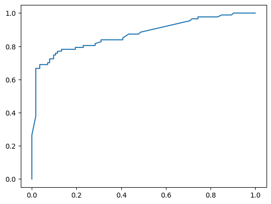
# 绘制ROC曲线
from sklearn.metrics import roc_curve
fpr, tpr, thres = roc_curve(y_test, y_pred_proba[:,1])
import matplotlib.pyplot as plt
plt.plot(fpr, tpr)
plt.show()
# AUC值
from sklearn.metrics import roc_auc_score
score = roc_auc_score(y_test, y_pred_proba[:,1])
score
0.8221950971416945
# 特征重要性
model.feature_importances_
array([1175, 668, 118, 895, 126])
features = X.columns  # 获取特征名称
importances = model.feature_importances_  # 获取特征重要性

# 通过二维表格形式显示
importances_df = pd.DataFrame()
importances_df['特征名称'] = features
importances_df['特征重要性'] = importances
importances_df.sort_values('特征重要性', ascending=False)
| 特征名称 | 特征重要性 | |
|---|---|---|
| 0 | 收入 | 1175 |
| 3 | 历史授信额度 | 895 |
| 1 | 年龄 | 668 |
| 4 | 历史违约次数 | 126 |
| 2 | 性别 | 118 |
12.5.4 模型参数调优
# 参数调优
from sklearn.model_selection import GridSearchCV  # 网格搜索合适的超参数
parameters = {

    'num_leaves': [10, 15, 31], 'n_estimators': [10, 20, 30], 'learning_rate': [0.05, 0.1, 0.2]}
model = LGBMClassifier()  # 构建分类器
grid_search = GridSearchCV(model, parameters, scoring='roc_auc', cv=5)  # cv=5表示交叉验证5次,scoring='roc_auc'表示以ROC曲线的AUC评分作为模型评价准则
# 输出参数最优值
grid_search.fit(X_train, y_train)  # 传入数据
grid_search.best_params_  # 输出参数的最优值
{'learning_rate': 0.2, 'n_estimators': 10, 'num_leaves': 10}
# 重新搭建分类器
model = LGBMClassifier(num_leaves=10, n_estimators=10,learning_rate=0.2)
model.fit(X_train, y_train)
LGBMClassifier(learning_rate=0.2, n_estimators=10, num_leaves=10)In a Jupyter environment, please rerun this cell to show the HTML representation or trust the notebook.
On GitHub, the HTML representation is unable to render, please try loading this page with nbviewer.org.
LGBMClassifier(learning_rate=0.2, n_estimators=10, num_leaves=10)
# 查看ROC曲线
y_pred_proba = model.predict_proba(X_test)
from sklearn.metrics import roc_curve
fpr, tpr, thres = roc_curve(y_test, y_pred_proba[:,1])
import matplotlib.pyplot as plt
plt.plot(fpr, tpr)
plt.show()
# 查看AUC值
y_pred_proba = model.predict_proba(X_test)
from sklearn.metrics import roc_auc_score
score = roc_auc_score(y_test, y_pred_proba[:, 1])
score
0.8712236801953005
12.6 LightGBM算法案例实战2 - 广告收益回归预测模型
12.6.1 案例背景
投资商经常会通过多个不同渠道投放广告,以此来获得经济利益。在本案例中我们选取公司在电视、广播和报纸上的投入,来预测广告收益,这对公司策略的制定是有较重要的意义。
12.6.2 模型搭建
# 读取数据
import pandas as pd
df = pd.read_excel('广告收益数据.xlsx')
df.head()
| 电视 | 广播 | 报纸 | 收益 | |
|---|---|---|---|---|
| 0 | 230.1 | 37.8 | 69.2 | 331.5 |
| 1 | 44.5 | 39.3 | 45.1 | 156.0 |
| 2 | 17.2 | 45.9 | 69.3 | 139.5 |
| 3 | 151.5 | 41.3 | 58.5 | 277.5 |
| 4 | 180.8 | 10.8 | 58.4 | 193.5 |
# 1.提取特征变量和目标变量
X = df.drop(columns='收益')
y = df['收益']

# 2.划分训练集和测试集
from sklearn.model_selection import train_test_split
X_train, X_test, y_train, y_test = train_test_split(X, y, test_size=0.2, random_state=123)

# 3. 模型训练和搭建
from lightgbm import LGBMRegressor
model = LGBMRegressor()
model.fit(X_train, y_train)
LGBMRegressor()In a Jupyter environment, please rerun this cell to show the HTML representation or trust the notebook.
On GitHub, the HTML representation is unable to render, please try loading this page with nbviewer.org.
LGBMRegressor()
12.6.3 Model prediction and evaluation
# 预测测试数据
y_pred = model.predict(X_test)
y_pred[0:5]
array([192.6139063 , 295.11999665, 179.92649365, 293.45888909,
       166.86159398])
# 预测值和实际值对比
a = pd.DataFrame()  # 创建一个空DataFrame
a['预测值'] = list(y_pred)
a['实际值'] = list(y_test)
a.head()
| Predictive value | actual value | |
|---|---|---|
| 0 | 192.613906 | 190.5 |
| 1 | 295.119997 | 292.5 |
| 2 | 179.926494 | 171.0 |
| 3 | 293.458889 | 324.0 |
| 4 | 166.861594 | 144.0 |
# 手动输入数据进行预测
X = [[71, 11, 2]]
model.predict(X)
array([140.00420258])
# 查看R-square
from sklearn.metrics import r2_score
r2 = r2_score(y_test, model.predict(X_test))
r2
0.9570203214455993
# 查看评分
model.score(X_test, y_test)
0.9570203214455993
# 特征重要性
model.feature_importances_
array([ 950, 1049, 963])
12.6.4 Model parameter tuning
# 参数调优
from sklearn.model_selection import GridSearchCV  # 网格搜索合适的超参数
parameters = {

    'num_leaves': [15, 31, 62], 'n_estimators': [20, 30, 50, 70], 'learning_rate': [0.1, 0.2, 0.3, 0.4]}  # 指定分类器中参数的范围
model = LGBMRegressor()  # 构建模型
grid_search = GridSearchCV(model, parameters,scoring='r2',cv=5) # cv=5表示交叉验证5次,scoring='r2'表示以R-squared作为模型评价准则
# 输出参数最优值
grid_search.fit(X_train, y_train)  # 传入数据
grid_search.best_params_  # 输出参数的最优值
{'learning_rate': 0.3, 'n_estimators': 50, 'num_leaves': 31}
# 重新搭建LightGBM回归模型
model = LGBMRegressor(num_leaves=31, n_estimators=50,learning_rate=0.3)
model.fit(X_train, y_train)

# 查看得分
model.score(X_test, y_test)
0.9558624845475153