[PyTorch Deep Learning] Predicting the inflow and outflow of shared bicycle trajectory data (with source code and data set)

If you need source code and data sets, please like and follow the collection and leave a private message in the comment area~~~

1. Data preprocessing and visualization

Shared bicycle data sets based on latitude and longitude, such as CitiBike, DivvyBike, etc. First, we perform simple analysis and preprocessing on the dataset and visualize it

Then, it further describes how to divide the entire city into a grid according to the latitude and longitude, regard the entire city as a "picture", and extract the spatio-temporal information of inflow and outflow in different areas of the city from the original GPS track data

Taking the CitiBik data in January 2015 as an example, first use Python3 and Pandas to read the data, and output the first 5 sample data

Because there are too many fields, we only take the required information fields and change the field names to make it more intuitive

Then use the Matplotlib library to count and visualize the usage frequency of shared bicycles at different latitudes and longitudes. This section takes the boarding point of passengers as an example, and the latitude and longitude interval is set to 0.002

The results are shown in the figure below. It can be found that the activity frequency of people in the city center is relatively high, which is in line with the laws of the real world. Frequency distribution of shared bicycle boarding points at different longitudes (left) and latitudes (right)

 Finally, we sample a portion of the data, analyze the spatial distribution of the data, and visualize it using a scatter plot

The results are shown in the figure below. Combined with the map of New York City, it can be found that most of the passengers who use shared bicycles are concentrated in the center of New York City, which is in line with objective laws. (horizontal axis: longitude, vertical axis: latitude)

Before we formally talk about the code, we first give a few necessary definitions to help us better understand the above concepts

Definition 1 (subregion): divide the city into m × n grids based on latitude and longitude, each grid is a subregion with equal size, use R=r_1,1,...,r_i,j,...,r_{_m ,n} to represent these sub-regions, where r_i, j represents the sub-region of the i-th row and j-th column

Definition 2 (incoming and outgoing "images"): Let P be a collection of shared bicycle trajectories, given a sub-region r_i, j, its corresponding inflow and outflow are defined as follows:

Where T_r:g_1→g_2→...→g_T_r is a sub-trajectory in P at the time interval t, g_l∈r_i,j means that g_l is located in the region r_i,j, and |⋅| represents the potential of the set. Define the inflow and outflow at time interval t as an adult flow tensor (Tensor) X^t∈ℛ^m×n×2, where X_i,j,0^t=x_in,i,j^t,X_i,j ,1^t=x_out,i,j^t

From the perspective of code, how to divide the original trajectory data based on GPS and model it into the above-mentioned inflow and outflow "image" data. First, import the required library, define the function geo_to_grid(), divide the city into grids, and the geo_to_grid() function returns the number of the sub-region

Then, define the bike_get_day_hour() function to parse the time field in the original trajectory to obtain the date and time of the current record

Combining the above data analysis with the pre-defined geo_to_grid() and bike_get_day_hour() functions, analyze the original trajectory data, divide the city into sub-regions with a time interval of 1 hour, and obtain the sub-regions of different time periods on different dates in the data set The incoming and outgoing flow data are stored in the pre-defined flow_array matrix, and finally the processed data is stored in the local current directory on a monthly basis

The bike_stat() function first reads the original trajectory data of CitiBike, extracts the original required information, such as time, latitude and longitude, etc., and sets the latitude and longitude filter conditions, that is, the latitude and longitude range of the city where it is located, and takes the data points outside the required latitude and longitude as abnormal points Delete, and then divide the city into grids, and obtain the starting point grid number, ending point grid number, date, time and other information of the corresponding trajectory data, and calculate the sub-area represented by each grid according to the above inflow and outflow formulas Inbound and outflow, and stored in the location corresponding to the matrix, and finally store the matrix locally in the current directory

2. Problem Statement and Model Framework

 Based on the public shared bicycle CitiBike dataset and New York taxi dataset NYCTaxi, a simple deep learning model based on migration learning is constructed for practical application and detailed explanation

In real applications, due to various reasons, such as backward data collection mechanism, data privacy protection, etc., the shared bicycle data we can obtain in some cities may be very limited, and some spatio-temporal data in cities are very rich, such as taxi data, etc. There is a spatiotemporal correlation between taxi data and shared bicycle data, and the knowledge contained in taxi data can be used to assist shared bicycles in predicting. This section uses the idea of ​​deep domain adaptation network in transfer learning and uses the Maximum Mean Discrepancy (MMD) , build a deep spatio-temporal domain adaptation network, from the perspective of data distribution, use the data-rich source domain city knowledge to assist the data-sparse target domain city, and predict the inflow and outflow of shared bicycles.

The model framework is shown in the figure:

Given a data-sufficient source domain and a data-sparse target domain, firstly a stacked 3D convolutional (Conv3D) network is used to map the original spatio-temporal shared bike data into a common embedding space, and then a fully connected network (FC) Learn the features unique to each domain, and embed these features into the Hilbert reproducible kernel space, use the maximum mean difference MMD as a constraint, reduce the difference between domains, so as to achieve the purpose of knowledge transfer, and finally, with the help of a layer of full Connect the network to make predictions

We assume that New York taxi data NYCTaxi is rich, and New York shared bicycle CitiBike data is sparse, so we use NYCTaxi as the source domain and CitiBike as the target domain. Specifically, we input all the NYCTaxi training data that has undergone data preprocessing into the model, and randomly sample a part CitiBike data for training

3. Data preparation

Using the CitiBike and NYCTaxi data for the whole year of 2015, with 1 hour as the time granularity, according to the above data preprocessing to generate regional-level inflow and outflow data, using the past 3 time steps to predict the data of the next 1 time step, for the source domain, Select the data of the first 300 days as the training set, randomly select the data of 64 time slices for the target domain in the first 300 days for training, the data of the next 32 days as the verification set, and the data of the last 32 days as the test set

First, integrate twelve months of data, make the required data set, and normalize it, rewrite __getitem__ and __len__ in torch.utils.data.Dataset to load our own data set. And after creating the Dataset class, use it with dataloader to continuously provide data to the model during model training

 4. Model Construction

In terms of model construction, this section mainly builds three networks:

SharedNet MMDNet  PredictNet

First, a SharedNet is established, using stacked 3D convolutional layers to learn the data representation of the original sequence of incoming and outgoing "images". 3D convolutions can be used to simultaneously capture spatial and temporal correlations. Sequence data for representation learning to encode spatiotemporal dependencies. All 3D convolutional layers are shared by data from both domains, thereby embedding source and target domains into a common latent representation space. Five layers of 3D convolutions are used in SharedNet Stacking, depending on the actual situation, the number of layers can be added or subtracted

In order to transfer the knowledge between the two domains, we use the idea of ​​​​the deep adaptive network DAN to input the characteristics of the source domain and the target domain learned by the 3D convolution layer into the deep adaptive network MMDNet established in this section. MMDNet consists of The stacked fully connected network is composed of the purpose of learning the characteristics of each domain. At the same time, the maximum mean difference MMD is used as a constraint for knowledge transfer. In order to learn the transferable features between the two domains, MMDNet embeds the data representation of each domain In the reproducible Hilbert space, and then use the maximum mean difference MMD as a constraint, through the gradient descent and back propagation algorithm, the distribution distance between the source domain and the target domain in the reproducible Hilbert space is shortened to achieve The purpose of knowledge transfer

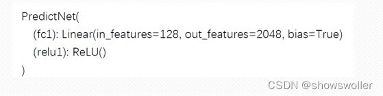
Finally, input the source domain features into PredictNet for prediction. PredictNet consists of a layer of fully connected network, and the number of layers can be added or subtracted depending on the situation.

5. Model training and testing

After the model is built, train the neural network and verify the model to save the relatively optimal model

First, set hyperparameters, such as learning rate, etc., and set the total number of epochs to 200

The root mean square error RMSE and the weighted sum of the maximum mean difference are used as the loss function, and the Adam optimizer is used to optimize the model. For each epoch, on the training set, input the data into the network learning features in batches, and make predictions, compare the predicted results with the real values, and use the designed loss function and gradient descent method to optimize the model

Then, the model is validated every few epochs, and if the result is better than last time, the better model is saved

The model testing part of the code is similar to the model validation part in the above code, but slightly different. The test process first needs to re-import the best model saved locally with the torch.load() function, and then use the load_state_dict() function to load the saved parameter dictionary into the model. At this time, the parameters in the model are the parameters in the training process. trained parameters

6. Model training process and result display

The SharedNet model shows:

The MMDNet model shows:

 

The PredictNet model shows:

 

The model training process shows:

 7. Code

 The last part of the code is as follows. If you need the source code and data set, please like and follow the collection and leave a private message in the comment area~~~

The preprocessing code is as follows

import numpy as np
import pandas as pd
import os
import multiprocessing as mul
import time
import warnings
warnings.filterwarnings('ignore')

# data_path与bike_bike可根据自身电脑数据集存储路径进行相应更改
data_path = '
bike_path ='
INTERVAL_NUM = 32
LNG_START = -74.02
LNG_STOP = -73.95
LNG_INTERVAL = abs(LNG_STOP - LNG_START) / INTERVAL_NUM
LAT_START = 40.67
LAT_STOP = 40.77
LAT_INTERVAL = abs(LAT_STOP - LAT_START) / INTERVAL_NUM


def geo_to_grid(geo):
    lat, lng = geo[0], geo[1]
    if (lat > LAT_STOP
            or lat < LAT_START
            or lng > LNG_STOP
            or lng < LNG_START
    ):
        return -1
    lng_ind = int(np.floor((lng - LNG_START) / LNG_INTERVAL))
    lat_ind = int(np.floor((lat - LAT_START) / LAT_INTERVAL))
    return lng_ind, lat_ind


def bike_get_day_hour(x):
    time_list = x.split(' ')
    date_str = time_list[0]
    date_list = date_str.split('/')
    time_str = time_list[1]
    day = int(date_list[1])
    hour = int(time_str.split(':')[0])
    return day, hour


def bike_stat(date_str):
    tl = []
    tl.append(time.time())
    df = pd.read_csv(data_path + '{}-citibike-tripdata.csv'.format(date_str), sep=',')
    tl.append(time.time())
    print('%s Data loaded in %.2fsec' %(date_str, (tl[-1]-tl[-2])))

    df_columns = [
        'starttime', 'stoptime',
        'start station longitude','start station latitude',
        'end station longitude', 'end station latitude'
    ]
    new_col_name = [
        'pick_up_time', 'drop_off_time',
        'pick_up_lon', 'pick_up_lat',
        'drop_off_lon', 'drop_off_lat'
    ]

    df = df.loc[:,df_columns]
    df.columns = new_col_name
    df_main = df[
        (LNG_START<df.pick_up_lon) & (df.pick_up_lon < LNG_STOP)
        & (LAT_START<df.pick_up_lat) & (df.pick_up_lat < LAT_STOP)
        & (LNG_START<df.drop_off_lon) & (df.drop_off_lon < LNG_STOP)
        & (LAT_START<df.drop_off_lat) & (df.drop_off_lat < LAT_STOP)
        ]


    df_main.pick_up_time = df_main.pick_up_time.apply(str)
    df_main.drop_off_time = df_main.drop_off_time.apply(str)
    with mul.Pool(48) as pool:
        pick_up_array = np.array(list(pool.map(bike_get_day_hour, df_main.pick_up_time)))
        drop_off_array = np.array(list(pool.map(bike_get_day_hour, df_main.drop_off_time)))
        start_grid_array = np.array(list(pool.map(geo_to_grid, df_main.loc[:, ["pick_up_lat", "pick_up_lon"]].values)))
        end_grid_array = np.array(list(pool.map(geo_to_grid, df_main.loc[:, ["drop_off_lat", "drop_off_lon"]].values)))
    tl.append(time.time())
    print('Get %s Using %.2f min' % (date_str, (tl[-1]-tl[-2])/60))
    df_main['start_x'] = start_grid_array[:, 0]
    df_main['start_y'] = start_grid_array[:, 1]
    df_main['end_x'] = end_grid_array[:, 0]
    df_main['end_y'] = end_grid_array[:, 1]
    df_main['start_day'] = pick_up_array[:, 0]
    df_main['start_hour'] = pick_up_array[:, 1]
    df_main['end_day'] = drop_off_array[:, 0]
    df_main['end_hour'] = drop_off_array[:, 1]

    start_g = df_main.groupby(['start_day','start_hour', 'start_x', 'start_y'])
    end_g = df_main.groupby(['end_day','end_hour', 'end_x', 'end_y'])
    start_count = start_g.agg('count').reset_index()
    end_count = end_g.agg('count').reset_index()
    print(date_str, 'have {} days which contains {} hours'.format(max(df_main.start_day), max(df_main.start_hour) + 1))
    flow_array = np.zeros((max(df_main.start_day), max(df_main.start_hour) + 1, INTERVAL_NUM, INTERVAL_NUM, 2))
    for row in start_count.iterrows():
        x_vle = row[1]['start_x']
        y_vle = row[1]['start_y']
        day = row[1]['start_day']-1
        hour = row[1]['start_hour']
        times = row[1]['end_day']
        try:
            flow_array[day, hour, x_vle, y_vle, 0] = times
        except:
            print(row[1])
    for row in end_count.iterrows():
        x_vle = row[1]['end_x']
        y_vle = row[1]['end_y']
        day = row[1]['end_day']-1
        hour = row[1]['end_hour']
        times = row[1]['start_day']
        try:
            flow_array[day, hour, x_vle, y_vle, 1] = times
        except:
            print(row[1])
    flow_array.tofile('./Data/CitiBike/' +'bike_%s' % date_str)
    print('%s Finished %.2f min' % (date_str, (tl[-1] - tl[-2]) / 60))
    print('*'*100)


def bike_count():
    global INTERVAL_NUM, LNG_START, LNG_STOP, LNG_INTERVAL
    global LAT_START, LAT_STOP, LAT_INTERVAL
    global data_path, taxi_path
    data_path = 'E:/CodingDocument/Pycharm/STMultiFlow/DataPreprocessing/DataSet/raw/Bike/'
    taxi_path = 'E:/CodingDocument/Pycharm/STMultiFlow/DataPreprocessing/DataSet/raw/Bike/'
    # taxi lng/lat
    INTERVAL_NUM = 32
    LNG_START = -74.02
    LNG_STOP = -73.95
    LNG_INTERVAL = abs(LNG_STOP - LNG_START) / INTERVAL_NUM
    LAT_START = 40.67
    LAT_STOP = 40.77
    LAT_INTERVAL = abs(LAT_STOP - LAT_START) / INTERVAL_NUM
    for year in range(2015, 2016):
        for mon in range(1, 13):
            if mon < 10:
                date_str = str(year) + '0' + str(mon)
            else:
                date_str = str(year) + str(mon)
            file_str = taxi_path+'bike_%s' % date_str
            if os.path.exists(file_str):
                print('bike_%s' % date_str + ' Exist!!!')
            else:
                bike_stat(date_str)


if __name__ == '__main__':
    bike_count()

training code

import numpy as np
import time
import torch
import torch.nn as nn
import torch.optim as optim
import matplotlib.pyplot as plt

from SrcDataLoader import *
from TgtDataLoader import *
from Shared_net import SharedNet
from model import MMDNet, PredictNet
from loss import *

data_split = [72*24, 20*24, 20*24]
# tgt_split = [32, 20*24, 20*24]
batch_size = 32

device = torch.device('cuda' if torch.cuda.is_available() else 'cpu')

# source_pretrain_dataset = PeopleDataset(mode='train', split=data_split)
# source_pretrain_loader = DataLoader(dataset=source_pretrain_dataset, batch_size=32, shuffle=True)

# source_prevalidate_dataset = PeopleDataset(mode='validate', split=data_split)
# source_prevalidate_loader = DataLoader(dataset=source_prevalidate_dataset, batch_size=32, shuffle=False)

# source_pretest_dataset = PeopleDataset(mode='test', split=data_split)
# source_pretest_loader = DataLoader(dataset=source_pretest_dataset, batch_size=32, shuffle=False)

src_train_dataset = NYCTaxiDataset(mode='train', split=data_split)
src_train_dataloader = DataLoader(dataset=src_train_dataset, batch_size=32, shuffle=True)

src_validate_dataset = NYCTaxiDataset(mode='validate', split=data_split)
src_validate_dataloader = DataLoader(dataset=src_validate_dataset, batch_size=32, shuffle=False)

src_test_dataset = NYCTaxiDataset(mode='test', split=data_split)
src_test_dataloader = DataLoader(dataset=src_test_dataset, batch_size=32, shuffle=False)

tgt_train_dataset = CitiBikeDataset(mode='train', split=data_split)
tgt_train_dataloader = DataLoader(dataset=tgt_train_dataset, batch_size=32, shuffle=False)

tgt_validate_dataset = CitiBikeDataset(mode='validate', split=data_split)
tgt_validate_dataloader = DataLoader(dataset=tgt_validate_dataset, batch_size=32, shuffle=False)

tgt_test_dataset = CitiBikeDataset(mode='test', split=data_split)
tgt_test_dataloader = DataLoader(dataset=tgt_test_dataset, batch_size=32, shuffle=False)

len_src_train = len(src_train_dataloader)
len_tgt_train = len(tgt_train_dataloader)

# lr = 0.0001
lr = 0.00001
l2_decay = 5e-4
num_epoches = 200

src_loss_list = []
total_loss_list = []
tgt_val_loss_list = []

seed = 32
np.random.seed(seed=seed)
torch.manual_seed(seed)
if device == 'cuda':
    torch.cuda.manual_seed(seed)

task_criterion = nn.MSELoss()

BaseNet = SharedNet().to(device)
# BaseNet.load_state_dict(torch.load('./Trained_model/best_model_normlization.pkl'))
TransferNet = MMDNet().to(device)
TaskNet = PredictNet().to(device)

for param in BaseNet.parameters():
    param.requires_grad = False

optimizer = optim.Adam([
    {'params': BaseNet.parameters()},
    {'params': TransferNet.parameters()},
    {'params': TaskNet.parameters()}], lr=lr, weight_decay=l2_decay)
best_rmse = 10000

for epoch in range(num_epoches):
    t0 = time.time()
    BaseNet.train()
    TransferNet.train()
    TaskNet.train()

    src_train_aver_rmse = 0
    mmd_loss = 0
    
    iter_src = iter(src_train_dataloader)
    iter_tgt = iter(tgt_train_dataloader)

    num_iter = len_src_train

    for i in range(0, num_iter):
        src_data_x, src_data_y = next(iter_src)
        tgt_data_x, tgt_data_y = next(iter_tgt)

        if (i+1) % len_tgt_train == 0:
            iter_tgt = iter(tgt_train_dataloader)
        
        src_data_x = src_data_x.float().to(device)
        src_data_y = src_data_y.float().to(device)
        tgt_data_x = tgt_data_x.float().to(device)
        tgt_data_y = tgt_data_y.float().to(device)

        optimizer.zero_grad()

        # print(src_data_x.shape, tgt_data_x.shape)
        
        inputs = torch.cat((src_data_x, tgt_data_x), dim=0)
        features = BaseNet(inputs)
        features = TransferNet(features)
        outputs = TaskNet(features)

        # print(outputs.shape, src_data_y.shape, inputs.size(0)/2)

        task_loss = torch.sqrt(task_criterion(outputs.narrow(0, 0, int(inputs.size(0)/2)), src_data_y))

        transfer_loss = DAN(features.narrow(0, 0, int(features.size(0)/2)), features.narrow(0, int(features.size(0)/2), int(features.size(0)/2)))

        total_loss = 0.1*transfer_loss + task_loss
        
        src_train_aver_rmse += total_loss.item()
        mmd_loss += transfer_loss.item()
        total_loss.backward()
        optimizer.step()
    src_train_aver_rmse /= len_src_train
    mmd_loss /= len_src_train
    src_loss_list.append(src_train_aver_rmse)
    total_loss_list.append(src_train_aver_rmse+mmd_loss)
    
    if (epoch+1) % 5 == 0 or epoch == 0:
        BaseNet.eval()
        TransferNet.eval()
        TaskNet.eval()
        tgt_validate_aver_rmse = 0
        len_tgt_validate = len(tgt_validate_dataloader)
        for i, (tgt_data_x, tgt_data_y) in enumerate(tgt_validate_dataloader):
            tgt_data_x, tgt_data_y = tgt_data_x.float().to(device), tgt_data_y.float().to(device)
            features = TransferNet(BaseNet(tgt_data_x))
            tgt_output = TaskNet(features)
            tgt_loss = torch.sqrt(task_criterion(tgt_output, tgt_data_y))
            tgt_validate_aver_rmse += tgt_loss.item()
        tgt_validate_aver_rmse /= len_tgt_validate
        tgt_val_loss_list.append(tgt_validate_aver_rmse)
        if tgt_validate_aver_rmse < best_rmse:
            best_rmse = tgt_validate_aver_rmse
            torch.save(BaseNet.state_dict(), 'best_BaseNet.pkl')
            torch.save(TransferNet.state_dict(), 'best_TransferNet.pkl')
            torch.save(TaskNet.state_dict(), 'best_TaskNet.pkl')
    t1 = time.time()
    print('Epoch: [{}/{}], Source train loss: {}, MMD loss: {}, tgt_best_validate_loss: {}, Cost {}min.'.format(epoch+1, num_epoches, src_train_aver_rmse, mmd_loss, best_rmse, (t1-t0)/60))

# loss_train_list = np.array(loss_train_list)
# loss_validate_list = np.array(loss_validate_list)
# np.save('loss_train_normlization.npy', loss_train_list)
# np.save('loss_validate_normlization.npy', loss_validate_list)

src_loss_list = np.array(src_loss_list)
total_loss_list = np.array(total_loss_list)
tgt_val_loss_list = np.array(tgt_val_loss_list)

np.save('src_loss_train_64hours.npy', src_loss_list)
np.save('total_loss_train_64hours.npy', total_loss_list)
np.save('tgt_loss_validate_64hours.npy', tgt_val_loss_list)

It's not easy to create and find it helpful, please like, follow and collect~~~