Common concepts in deep learning (convergence, optimizer, learning rate, etc.)

1. Convergence

To make a simple analogy, training a network model is like solving an equation. In order to get the extreme point of this equation, the training process is like finding a direction and constantly approaching this direction, so that the value of the equation continues to decrease. Eventually it reaches the extreme point without convergence, that is, no matter how you run, the solution of the equation will not decrease. That is, the last extreme point cannot be reached. In terms of loss, it shows that the stability is relatively large. Similar to iteration failure or system instability, up and down fluctuations cannot approach a fixed value.

Convergence means that a certain value has been approaching the threshold we expect. Take the loss loss in deep learning as an example. The following picture is a graph of loss during each round of training. You can see that loss has been From the beginning of 1.8 to 1.0, 1.0 is the threshold we expect, and 1.8 is the maximum loss value at the beginning.

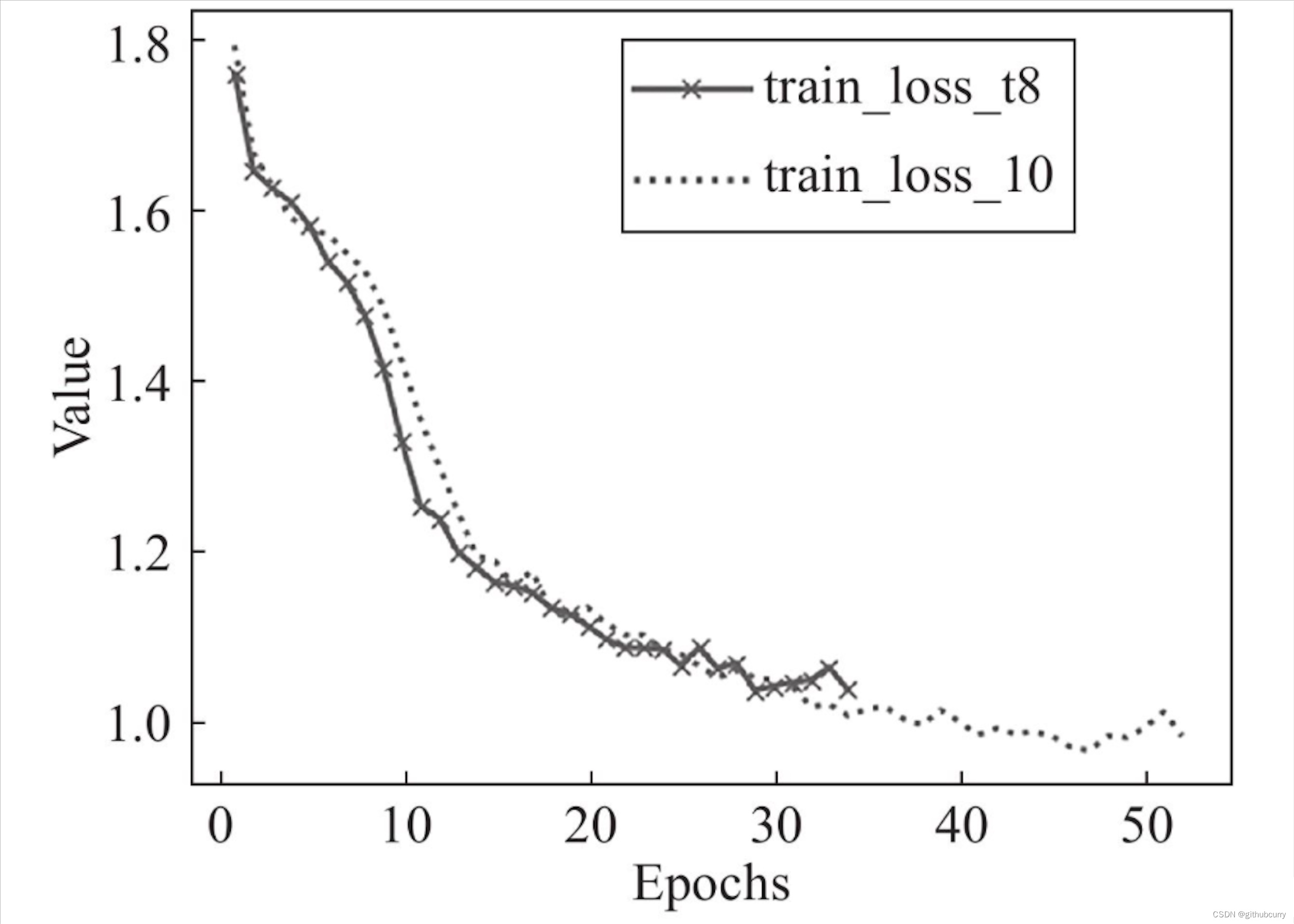
It can be seen that the loss value has been approaching our expected threshold during the training process. This curve is very smooth, and there is no reason why the curve has been stuck at a certain point and does not fall or suddenly rises (in this case, it is running away). , if there may be a problem with the learning rate setting. As shown below:

It can be seen that it suddenly increased back during the original decline. This reason may be that there is a problem when your learning rate decays. Such a loss value will definitely have an impact when updating the weight. This situation is also called local oscillation. That is, jumping back and forth around a specific threshold, and jumping back and forth between the thresholds of 1.0 is always iterative. In this case, there is a problem of inability to converge.

The learning rate represents the utilization rate of your loss value, so your loss decay depends on your learning rate. The intuitive manifestation of the non-convergence of the network is that the loss function cannot be reduced. In essence, there is a problem with the network or the training method, including the bachsize size, whether the data is normalized, the learning rate design, the initialization weight, etc., all of which need to be checked.

2. Optimizer

2.1 What is an optimizer

The optimizer is a tool to guide the neural network to update the parameters. After the deep learning calculates the loss function, it needs to use the optimizer to perform backpropagation to complete the update of the network parameters. In this process, an optimizer will be used, and the optimizer can use computer numerical calculation methods to obtain the network parameters with the smallest loss function. In deep learning, different optimizers just define different first-order momentum and second-order momentum. The first-order momentum is a function related to the gradient, and the second-order momentum is a function related to the square of the gradient. Commonly used optimizers mainly include stochastic gradient descent (SGD), Momentum, AdaGrad, RMSProp and Adam optimizers.

2.1.1 Backpropagation

Backpropagation is to let the neural network update the previous parameters. It can be imagined as when doing a question (the question can be thought of as a neuron node one by one), we have done right, and some have done wrong. It can in turn tell us which piece of knowledge we should focus on learning and which question types to learn, and then the neural network increases the parameter weight of this node through forward, which is the direction propagation update parameter

The optimizer or optimization algorithm minimizes (maximizes) the loss function by training the optimization parameters. The loss function is used to calculate the degree of deviation between the real value and the predicted value of the target value Y in the test set.

In order to make the model output approach or reach the optimal value, we need to use various optimization strategies and algorithms to update and calculate network parameters that affect model training and model output.

2.2 Gradient descent method

For the optimization algorithm, the goal of optimization is the parameter θ in the network model (it is a set, θ1, θ2, θ3...) The objective function is the loss function L = 1/N ∑ Li (the superposition and mean value of each sample loss function). The L variable of this loss function is θ, where the parameters in L are the entire training set. In other words, the objective function (loss function) is determined through the entire training set. If the full training set is different, the image of the loss function will be different. So why can't optimization be performed if a saddle point/local minimum point is encountered in the mini-batch? Because at these points, the gradient of L with respect to θ is zero, in other words, the partial derivative is calculated for each component of θ, and brought into the full training set, the derivative is zero. For SGD/MBGD, the loss function used each time is only determined by this small batch of data, and its function image is different from the real loss function of the complete set, so the gradient it solves also contains a certain degree of randomness. In the saddle point Or at the local minimum point, the shock jumps, because at this point, if the entire training set is brought in, that is, BGD, the optimization will stop. If it is mini-batch or SGD, the gradient found each time is different. Yes, it will vibrate and jump back and forth.

2.3 Common optimizers:

• Batch Gradient Descent （BGD）
• Stochastic Gradient Descent (SGD)
• Mini-Batch Gradient Descent （MBGD）
• Momentum
• Nesterov Accelerated Gradient
• Adagrad （Adaptive gradient algorithm）
• Adadelta
• RMS plug
• Adam：Adaptive Moment Estimation

2.4 Comparison of optimizer effects

Let's take a look at the performance of several algorithms on saddle points and contour lines:


In the above two cases, it can be seen that Adagrad, Adadelta, and RMSprop almost quickly find the right direction and move forward, and the convergence speed is quite fast, while other The method is either very slow, or it takes a lot of detours to find it. It can be seen from the figure that the adaptive learning rate methods, namely Adagrad, Adadelta, RMSprop, Adam, will be more suitable and have better convergence in this scenario.

2.5 How to choose an optimization algorithm

• If the data is sparse, use adaptive methods, ie Adagrad, Adadelta, RMSprop, Adam.

• RMSprop, Adadelta, Adam are similar in many cases.

• Adam added bias-correction and momentum on the basis of RMSprop,

• Adam performs better than RMSprop as the gradient becomes sparser.

• Overall, Adam is the best choice.

• SGD is used in many papers, without momentum and so on. Although SGD can reach the minimum value, it takes longer than other algorithms and may be trapped in saddle points.

• If you need faster convergence, or train a deeper and more complex neural network, you need to use an adaptive algorithm.

3. Learning rate

The first step in parameter tuning is to know what this parameter is and how its changes affect the model. Every machine learning researcher will face the test of the parameter tuning process, and in the parameter tuning process, the adjustment of the learning rate is a very important part.

3.1 What is the learning rate

To understand what the learning rate is, you must first understand the mechanism of neural network parameter update, gradient descent + backpropagation:

To sum up one sentence: the output error is backpropagated to the network parameters to fit the output of the sample. It is essentially a process of optimization, which gradually tends to the optimal solution.

However, how much error is used for each update parameter needs to be controlled by a parameter, which is the learning rate (Learning rate), also known as the step size.

The learning rate represents the rate at which information is accumulated in a neural network over time. Learning rate is one of the most performance-impacting hyperparameters, and if we could only tune one hyperparameter, it would be the best choice. Compared with other hyperparameters, the learning rate controls the effective capacity of the model in a more complicated way. When the learning rate is optimal, the effective capacity of the model is the largest. Therefore, in order to train a neural network, one of the key hyperparameters that needs to be set is the learning rate.

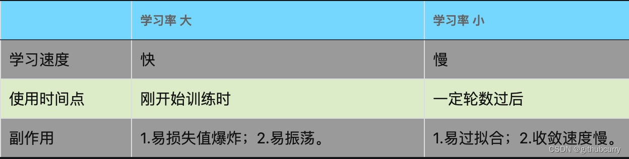
3.2 The influence of learning rate on the model

The larger the learning rate, the greater the impact of the output error on the parameters, and the faster the parameters are updated, but at the same time, the greater the impact of abnormal data, it is easy to diverge.

Learning rate (Learning rate, η) is an important hyperparameter in supervised learning and deep learning, which determines whether the objective function can converge to a local minimum and when to converge to the minimum.

An appropriate learning rate can make the objective function converge to a local minimum within an appropriate time.

When using the gradient descent algorithm for optimization, in the weight update rule, a coefficient will be multiplied before the gradient term, and this coefficient is called the learning rate α.

The learning rate is a hyperparameter that guides us how to use the gradient of the loss function to adjust the weights of the network in the gradient descent method.
new_weight = old_weight - learning_rate * gradient

3.3 Effect of learning rate on loss value and deep network

• If the learning rate is too large, the loss function may directly cross the global optimal point, prone to gradient explosion, loss vibration amplitude is large, and the model is difficult to converge.
• If the learning rate is too small, the change speed of the loss function is very slow, and it is easy to overfit. will greatly increase the convergence complexity of the network. While using a low learning rate ensures that we do not miss any local minima, it also means that we will take longer to converge, especially if we are stuck at a local optimum when.

3.4 The role of learning rate

The learning rate controls the learning progress of the model.

It can be seen from the above that choosing a good learning rate update strategy for a deep network can be abstracted into the following two benefits:

• Reach the minimum value of loss faster
• The loss value that guarantees convergence is the global optimal solution of the neural network

3.5 Learning rate setting

The ideal learning rate is not a fixed value, but a value that changes with the number of training decays, that is, in the early stage of training, the learning rate is relatively large, and as the training progresses, the learning rate continues to decrease until the model converges.

During the training process, a dynamically changing learning rate is generally set according to the number of training rounds:

• At the beginning of training: the appropriate learning rate is 0.01 ~ 0.001.
• After a certain number of rounds: Gradually slow down.
• Near the end of training: The decay of the learning rate should be more than 100 times.

In the current research, the commonly agreed learning rate setting standard is: first set a large learning rate to make the loss value of the network drop rapidly, and then reduce the learning rate a little bit with the increase of the number of iterations to prevent the global optimal solution .

So we now face two problems:

How to choose the initial learning rate?

• The initial value of the learning rate of most networks is set to 0.01 and 0.001.
• A more scientific setting method: first set a very small learning rate, increase the learning rate after each epoch, and record the loss or acc of each epoch, the more iterative epochs, the higher the learning rate to be tested More, and finally compare the loss or acc corresponding to different learning rates.
• How to update the learning rate according to the number of iterations (i.e. decaying learning rate strategy)

3.5.3 Learning rate size

3.5.2 Learning rate mitigation mechanism

From the initial learning rate to continuously decay downward, the strategy generally has the following three methods: round decay, exponential decay, and score decay

• The number of rounds is slowed down: if the learning rate is halved after five rounds of training, it will be halved again after the next five rounds;
• Exponential slowdown: that is, the learning rate increases exponentially according to the number of training rounds, etc.;
• Score slowing down

3.6 Learning rate and objective function loss value curve

Ideally, the curve should be a downward slide [green line] :

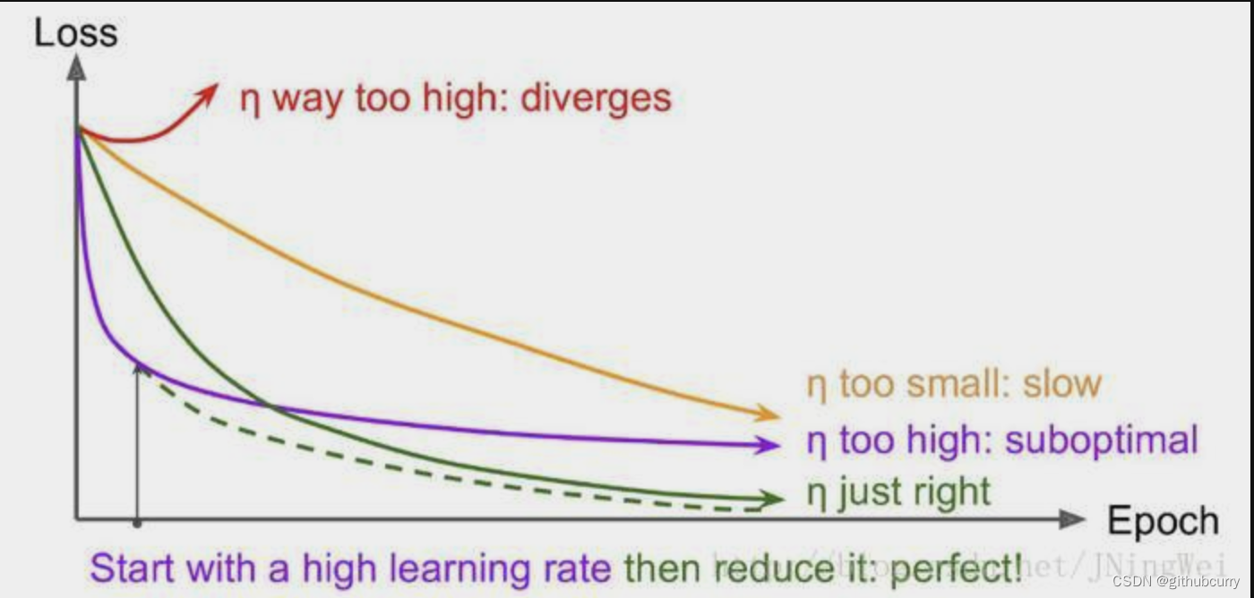
• The curve rises at the beginning [red line]:
  Solution: The initial learning rate is too large, resulting in oscillation. The learning rate should be reduced and the training should be started from scratch.
• The curve dropped strongly at the beginning, and returned to the level after a short time [purple line]:
  Solution: The learning rate in the later stage is too large, which makes it impossible to fit. The learning rate should be reduced and the next few rounds of training should be retrained.
• The whole curve is slow [yellow line]:
  Solution: The initial learning rate is too small, resulting in slow convergence. You should increase the learning rate and start training from scratch.

3.7 Learning rate summary

Choosing the optimal learning rate is important because it determines whether the neural network can converge to the global minimum. Choose a higher learning rate, it can have undesired consequences on your loss function, so the global minimum is almost never reached because you are likely to skip it. So, you're always around the global minimum, but never converged to the global minimum. Choosing a small learning rate will help the neural network converge to the global minimum, but it will take a lot of time - because you are only making very little adjustments in the weights of the network. This way you have to spend more time training the neural network. A smaller learning rate is also more likely to trap the neural network in a local minimum, that is, the neural network will converge to a local minimum, and because the learning rate is small, it will not be able to jump out of the local minimum. So, you have to be very careful when setting the learning rate. The figure below visualizes this problem:

the optimal optimal learning rate is related to the loss function map (loss landscape) of the neural network, which is a function of the network parameter value, when performing inference (prediction) on a specific data set, quantization and The associated "error" is configured using specific parameters. This loss map may look very different for very similar network architectures. The optimal learning rate depends on the topology of your loss map, i.e. your model structure and dataset. While you can use the default learning rate (determined automatically by your deep learning library) to provide a similar result, you can also improve performance by searching for an optimal learning rate.

Ultimately, we want to get a learning rate that greatly reduces the network loss. We can observe this by doing a simple experiment while gradually increasing the learning rate for each mini-batch (iteration), recording the loss after each increment. This gradual increase can be linear or exponential.

For too slow a learning rate, the loss function may decrease, but at a very shallow rate. When entering the optimal learning rate region, you will observe a very large drop in the loss function. Increasing the learning rate further can cause the loss function value to "jump around" or even diverge around the lowest point. Remember, the best learning rate is paired with the steepest descent on the loss function, so we're mainly concerned with the slope of the analysis graph. As shown in the figure below:

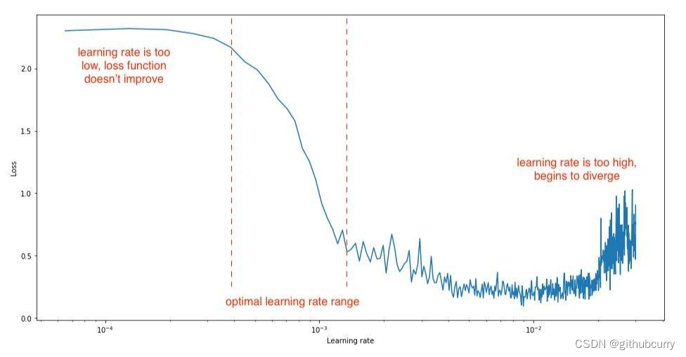
you should set your learning rate bounds for this experiment so that you can see all three stages, making sure to identify the optimal range.

Another commonly used technique is learning rate annealing. It is recommended that you start with a relatively high learning rate and then slowly reduce the learning rate during training. The idea behind this approach is that we like to quickly move from initial parameters to a range of "good" parameter values, but then we want a learning rate small enough that we can explore "deeper and narrower places in the loss function", (From Karparthy's CS231n course notes: http://cs231n.github.io/neural-networks-3/#annealing-the-learning-rate). The reason for this is mainly that, as mentioned earlier, too high a learning rate can cause parameter updates to "jump around" between the minimum and subsequent updates, which can lead to constant noise in the minimum range convergence, or in more extreme cases may cause divergence from the minimum.

The most popular way of learning rate annealing is "Step Decay", where the learning rate is decreased by a certain percentage after a certain number of training epochs. Other

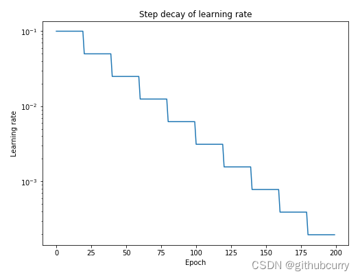
methods are periodic learning rate tables, or using Stochastic Gradient Descent (SGDR), etc.

4. Hyperparameters

In the context of machine learning (including deep learning), a hyperparameter is a parameter whose value is set before starting the learning process, rather than the parameter data obtained through training. Usually, it is necessary to optimize the hyperparameters and select a set of optimal hyperparameters for the learning machine to improve the performance and effect of learning.

4.1 Hyperparameters usually exist in:

1. Define higher-level concepts about the model, such as complexity or learning ability.
2. Cannot be learned directly from data during standard model training and needs to be pre-defined.
3. can be determined by setting different values, training different models and choosing better test values

Specifically, the learning rate (learning rate), the number of gradient descent method iterations (iterations), the number of hidden layers (hidden layers), the number of hidden layer units, and the activation function (activation function) in deep learning all need to be based on the actual situation. to set, these numbers actually control the value of the final parameter sum, so they are called hyperparameters.

4.2 Finding the optimal value of hyperparameters

Hyperparameters need to be set manually, and the set values ​​have a great impact on the results. Common methods for setting hyperparameters are:

• Guess and check: Choose parameters based on experience or intuition, iterating all the way.
• Grid search: Let the computer try a set of values ​​evenly distributed within a certain range.
• Random Search: Let the computer pick a set of values ​​at random.
• Bayesian optimization: Using Bayesian optimization hyperparameters, you will encounter the difficulty that the Bayesian optimization algorithm itself requires many parameters.

4.3 Hyperparameter Search Process

The general process of hyperparameter search is as follows:

1. Divide the dataset into training set, validation set and test set.
2. Optimize the model parameters on the training set according to the performance indicators of the model.
3. The hyperparameters of the model are searched on the validation set according to the performance indicators of the model.
4. Step 2 and Step 3 are alternately iterated to finally determine the parameters and hyperparameters of the model, and verify the pros and cons of the evaluation model in the test set.
5. Among them, the search process requires search algorithms, generally including: grid search, random search, heuristic intelligent search, Bayesian search, etc.