The basic theory of GCN

Practical basic theory of GCN (for coding)

1. Representation of graphs

$$\begin{array}{rl}& A:\; adjacency\; matrix\; of\; graph\; structure\\ & \tilde{A}:\; adjacency\; matrix\; with\; self-connection\\ & \tilde{A}=A+I\\ & \tilde{D}:\; degree\; matrix\; of\; adjacency\; matrices\; with\; self-connections\\ & {\tilde{D}}_{ii}=\sum _j{\tilde{A}}_{ij}\\ & H:\; characteristics\; of\; graph\; nodes\\ & l:Neural\; Network\end{array}$$

2. The principle of GCN

$$H^{(l+1)}=d({\tilde{D}}^{-1/2}\tilde{A}{\tilde{D}}^{-1/2}{H}^{(l)}{W}^{(l)})$$

• The input of GCN is the adjacency matrix A and the node feature H, directly do the inner product, then multiply a parameter matrix W, and then activate it, isn't it equivalent to a neural network layer? Why have a self-connected adjacency matrix?
  Hint: It is impossible to distinguish between "self-node" and "no-connection node". If only A is used, since the diagonal of A is all 0, when multiplying with the feature matrix H, only the weighted sum of the features of all neighbors of a node will be calculated, and the features of the node itself will be ignored. .

• Why do you need a degree matrix with a self-connected adjacency matrix?
  Tip: A is a matrix that has not been normalized, so multiplying it with the feature matrix H will change the original distribution of the feature, so do a normalization process on A. The importance of nodes with a large degree of balance. (symmetric normalized Laplacian matrix)
  $$Norm{A}_{ij}=\frac{A_{ij}}{\sqrt{d_i}\sqrt{d_j}}$$

3. The underlying implementation of GCN (pytorch)

Pytorch-Geometric (PyG)：https://github.com/pyg-team/pytorch_geometric

Official documentation https://pytorch-geometric.readthedocs.io/en/latest/notes/introduction.html

PyG provides the following main functions:

• Data Handling of Graphs (graph data processing)
• Common Benchmark Datasets (common benchmark datasets)
• Mini-batches
• Data Transforms (data conversion)
• Learning Methods on Graphs (graph learning algorithm)
• Exercises _

3.1 Data Handling of Graphs (graph data processing)

Graphs are used to model pairwise relationships (edges) between objects (nodes). A single graph in PyG is described by an instance of torch_geometric.data.Data, which by default contains the following properties:

• data.x: node feature matrix H, shape:[num_nodes, num_node_features]
• data.edge_index: graph adjacency matrix A, shape: [2, num_edges], data type:torch.long

  For example: [[0,1,1,2],[1,0,2,1]]: indicates that there is an edge between node 0 and node 1, and an edge between node 1 and node 2,
  namely: [[all starting points node], [all endpoint nodes]]. This is different from general thinking, they are transposed of each other. Note that when using it, it must be converted to this form before use

• data.edge_attr: edge feature matrix, shape:[num_edges, num_edge_features]
• data.y: training target (can be any shape), eg , label on node scale, shape: [num_nodes, *]or label on whole graph scale[1, *]
• data.pos: node coordinate matrix, shape:[num_nodes, num_dimensions]

import torch
from torch_geometric.data import Data

# 注意：edge_index是定义所有边的源节点和目标节点的张量，不是索引元组的列表。
# --------------------第一种定义方法-----------------------------
edge_index = torch.tensor([[0, 1, 1, 2],
                           [1, 0, 2, 1]], dtype=torch.long)
x = torch.tensor([[-1], [0], [1]], dtype=torch.float)

data = Data(x=x, edge_index=edge_index)
>>> Data(edge_index=[2, 4], x=[3, 1])

# --------------------第二种定义方法-----------------------------
edge_index = torch.tensor([[0, 1],
                           [1, 0],
                           [1, 2],
                           [2, 1]], dtype=torch.long)
x = torch.tensor([[-1], [0], [1]], dtype=torch.float)

data = Data(x=x, edge_index=edge_index.t().contiguous()) # 注意这里edge_index进行了转置
>>> Data(edge_index=[2, 4], x=[3, 1])

3.2 Common Benchmark Datasets

Contains some basic datasets used for testing

3.3 Mini-batches

Neural networks are usually trained in a batch fashion. PyG parallelizes mini-batches by creating a sparse block-diagonal adjacency matrix (defined by 'edge_index') and concatenating the feature and target matrices in the node dimension.

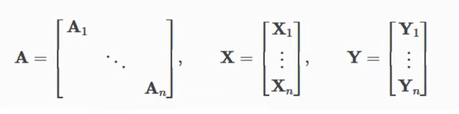
This combination allows different numbers of nodes and edges in a batch example (i.e. A1~An their dimensions can be different):

4. Implement the GCN layer

This formula can be broken down into the following steps:

1. Add self-loops in the adjacency matrix.
2. Linearly transform the node feature matrix.
3. Calculate the normalization coefficient.
4. Normalize node features
5. Summing adjacent node features (“add” aggregation).

import torch
from torch_geometric.nn import MessagePassing
from torch_geometric.utils import add_self_loops, degree

class GCNConv(MessagePassing):
    def __init__(self, in_channels, out_channels):
        super().__init__(aggr='add')  # "Add" aggregation (Step 5).
        self.lin = torch.nn.Linear(in_channels, out_channels)

    def forward(self, x, edge_index):
        # x has shape [N, in_channels]
        # edge_index has shape [2, E]

        # Step 1: 在邻接矩阵中添加自循环。~A
        edge_index, _ = add_self_loops(edge_index, num_nodes=x.size(0))

        # Step 2: 线性变换节点特征矩阵。H*W
        x = self.lin(x)

        # Step 3: 计算归一化系数。
        row, col = edge_index # row：第一行数据，col：第二行数据
        deg = degree(col, x.size(0), dtype=x.dtype) # deg：度矩阵D; 参数为col算入度，参数为row算出度
        deg_inv_sqrt = deg.pow(-0.5) # D^(-0.5)
        deg_inv_sqrt[deg_inv_sqrt == float('inf')] = 0
        # The result is saved in the tensor norm of shape [num_edges, ]
        norm = deg_inv_sqrt[row] * deg_inv_sqrt[col] # D^(-0.5) * ~A * D^(-0.5)

        # Step 4-5: 规范化节点特征，对相邻节点特征求和(“add”聚合)。
        return self.propagate(edge_index, x=x, norm=norm) # D^(-0.5) * ~A * D^(-0.5) * H * W

    def message(self, x_j, norm): # 扩展相乘，保证A和H能够相乘
        # x_j has shape [E, out_channels]

        # Step 4: Normalize node features.
        return norm.view(-1, 1) * x_j

5. Simple example of GCN

import torch
import torch.nn.functional as F
from torch_geometric.nn import GCNConv

class GNN(torch.nn.Module):
    def __init__(self):
        super().__init__()
        self.conv1 = GCNConv(dataset.num_node_features, 16) # 参数1: 节点特征数，参数2: 随机
        self.conv2 = GCNConv(16, dataset.num_classes) # 参数1: 与上一层一致，参数2: label类别数

    def forward(self, data):
        x, edge_index = data.x, data.edge_index
        
        x = self.conv1(x, edge_index) # x为特征矩阵，edge_index为邻接矩阵
        x = F.relu(x)
        x = F.dropout(x, training=self.training)
        x = self.conv2(x, edge_index)

        return F.log_softmax(x, dim=1)

from torch_geometric.datasets import Planetoid
dataset = Planetoid(root='./data/Cora', name='Cora')

device = torch.device('cuda' if torch.cuda.is_available() else 'cpu')
model = GNN().to(device)
data = dataset[0].to(device)
optimizer = torch.optim.Adam(model.parameters(), lr=0.01, weight_decay=5e-4)

model.train()
for epoch in range(200):
    optimizer.zero_grad()
    out = model(data)
    loss = F.nll_loss(out[data.train_mask], data.y[data.train_mask])
    loss.backward()
    optimizer.step()

model.eval()
pred = model(data).argmax(dim=1)
correct = (pred[data.test_mask] == data.y[data.test_mask]).sum()
acc = int(correct) / int(data.test_mask.sum())
print(f'Accuracy: {
      
      acc:.4f}')

Mathematical theoretical basis of GCN (for understanding)

1. GCN foundation

GNN公式： $H^{(l+1)}=f(A,H(l))$ , where$A$ is graph adjacency matrix,$H$ is the characteristic matrix of all nodes on the graph

GCN公式：$H^{(l+1)}=d\left({\hat{D}}^{-1/2}\hat{A}{\hat{D}}^{-1/2}{H}^{\left(l\right)}\theta \right)$, where$D$ is the degree matrix,$\theta$ is the parameter to be learned

The difference between GNN and GCN:

GNNs include:

1. Direct processing of graphs from the airspace
2. First convert the graph from the spatial domain to the spectral domain, and then convert to the spatial domain after the spectral domain operation is completed. Namely GCN . As for why it is necessary to convert from the spatial domain to the spectral domain, it is because the structure of the nodes on the graph is not fixed in the spatial domain (for example, the adjacent nodes of the nodes on each graph are inconsistent), so it is difficult to find a general convolution. Check the image to extract features, but convert it to the spectral domain, which is easy to handle. This is why the idea of ​​Fourier transform is used.

Let's explore the source of the following GCN formula.

2. Spectral Domain Graph Theory

In short, the spectral domain graph theory is a theory that studies some properties of the correlation matrix with the adjacency matrix A.

First, review a few related concepts in linear algebra:

(1) Eigenvalues ​​and eigenvectors

For a matrix A, if $A\vec{x}=l\vec{x}$, and $|\vec{x}|\ne 0$ , then$\vec{x}$Is the eigenvector of A, $\lambda$ is a corresponding eigenvalue

(2) Real symmetric matrix: The elements of the matrix are all real numbers, and the matrix is ​​a symmetric matrix.

Properties of real symmetric matrices : The eigenvectors corresponding to different eigenvalues ​​of real symmetric matrix A are orthogonal . Written as a mathematical expression, A can be expressed as $A=U\Lambda U^T$ ,withUUT$U\; U{U}^T=I$ ,$\Lambda$ is a matrix whose diagonal elements are all eigenvalues ​​and other positions are 0.

(3) Positive semi-definite matrix:

Properties of positive semi-definite matrices: The matrix is ​​a real symmetric matrix; all eigenvalues ​​of the matrix are greater than or equal to 0

（4）二次型：${\vec{x}}^{T}A\vec{x}$
（5）Rayleigh商：${\vec{x}}^{T}A\vec{x}/{\vec{x}}^T\vec{x}$. Properties: when $\vec{x}$When is the eigenvector of A, the Rayleigh quotient is the corresponding eigenvalue.

With the above theories, let's take a look at some matrices related to the adjacency matrix A:

Laplace matrix: $L=D-A$ ,$whereDis\; the\; degree\; matrix$
symmetric normalized Laplacian matrix: $L_{sym}=D^{-1/2}L{D}^{-1/2}$

Why study the above two matrices? It is because these two matrices have excellent properties (these properties can be applied to the Fourier transform). The properties are as follows:

1. Both matrices are real symmetric matrices (and therefore positive semi-definite matrices), so there are n eigenvalues ​​and corresponding eigenvectors greater than or equal to zero.
2. $L_{sym}$The value range of the eigenvalue is [0,2]

The first property does not need to be proved, because the relevant properties of the matrix have been given above. Let's prove the second property:

1. First define a matrix G, where (i,i), (i,j), (j,i), (j,j) are 1, and other positions are 0, the form is as follows: 0 0 0 . . . 0 0
   $$\begin{array}{ccccccc}0& 0& 0& ...& 0& 0& 0\\ 0& 0& 0& ...& 0& 0& 0\\ 0& 0& 1& ...& 1& 0& 0\\ ...& & & & & & \\ 0& 0& 1& ...& 1& 0& 0\\ 0& 0& 0& ...& 0& 0& 0\\ 0& 0& 0& ...& 0& 0& 0\end{array}$$
2. Then calculate ${\vec{x}}^{T}G\vec{x}$, where $\vec{x}$For any vector, the result is $${\vec{x}}^{T}G\vec{x}=(x_i+x_j{)}^2$$ (I won’t expand it here, you can calculate it on the draft paper yourself)
3. Define a $L^{pos}=D+A$，易得 $$L^{pos}=D+A=\sum _{i,j\in E}G$$ (the following summation formula is the addition of the G matrix in all cases)
4. Then you can get ${\vec{x}}^T{L}^{pos}\vec{x}={\sum }_{i,j\in E}(x_i+x_j{)}^2$
5. 定义 $L_{sym}^{pos}=D^{-1/2}{L}^{pos}{D}^{-1/2}=D^{-1/2}(D+A)D^{-1/2}=I+D^{-1/2}A{D}^{-1/2}$。
6. 又因为 ${\vec{x}}^T{L}_{sym}^{pos}\vec{x}={\vec{x}}^T(I+D^{-1/2}A{D}^{-1/2})\vec{x}>=0$ , so after expanding the transformation, you can get
   $${\vec{x}}^T{L}_{sym}\vec{x}/{\vec{x}}^T\vec{x}<=2$$
7. It is found that the left side of the equal sign is the Rayleigh quotient. According to the properties of the Rayleigh quotient mentioned above, when $\vec{x}$The eigenvector of the matrix is, and the value of the corresponding Rayleigh quotient is the eigenvalue, so the above expression is $L_{sym}$All eigenvalues ​​of are less than or equal to 2.
8. And because $L_{sym}$is a positive semidefinite matrix, so the eigenvalues ​​are greater than or equal to 0. Therefore $L_{sym}$The range of eigenvalues ​​is [0,2].

This property is very important and will be used below.
Let's discuss the knowledge of Fourier transform used in graph convolution.

3. Fourier transform

First of all what is the Fourier transform? Let's understand it from the following picture: Suppose we have a function f ( t ) f(t)

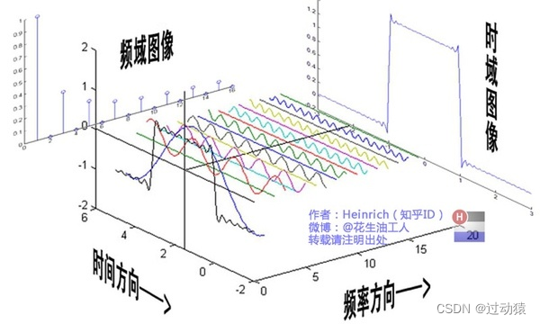
that describes sound waves in time$f\left(t\right)$ , then the function of Fourier transformis to decompose this function into multiple sinusoidal functions that also take time as an independent variable. is the mathematical principle of Fourier transform, which will not be discussed here), and then put these functions on another coordinate system with the amplitude as the ordinate and the frequency as the abscissa. To put it simply, the original function is the left view of the above image (ie, the instant domain image), and the transformed function is the right view of the above image (ie, the frequency domain image).

Why do such transformations? Because in some tasks, if we deal with the problem in the time domain, it will be very troublesome, but it will be very simple to deal with the problem in the frequency domain. For example, a man and a woman talk at the same time (as we all know, the frequency of boys’ voices is low, and the frequency of girls’ voices is high), we have obtained this audio, but we want to remove the voice of boys in this audio, if only based on the time domain image Processing will be It is very troublesome, but if we can map this wave to the frequency domain, then the sound waves of boys will be concentrated in the low frequency band, and the sound waves of girls will be concentrated in the high frequency band, so we can directly delete the sound waves of the low frequency band. This is very simple.

Reflected on the figure, it is difficult for us to solve the problem in the airspace, so we need to change this problem to another coordinate system to solve (that is, the spectral domain), and then convert the result back to the airspace. This is the idea of ​​Fourier transform used in GCN.

Having said so many conceptual things, let's talk about mathematical theory:

First define $\vec{c}$is a certain eigenvector of all nodes in the graph, and then explore $L\vec{c}$meaning of:

1. 首先$L=D-A$，因此$L\vec{c}=(D-A)\vec{c}=D\vec{c}-A\vec{c}$。
2. Then calculate $D\vec{c}$和$A\vec{c}$, and then do the difference, you can get (the right side is a matrix of n*1)
   $$L\vec{c}=\begin{array}{c}{\sum }_{x_j\in and{x}_{1}Adjacent}(x_1-x_j)\\ {\sum }_{x_j\in and{x}_{2}Adjacent}(x_2-x_j)\\ {\sum }_{x_j\in and{x}_{1}Adjacent}(x_1-x_j)\\ ...\\ {\sum }_{x_j\in and{x}_{1}Adjacent}(x_1-x_j)\end{array}$$
3. We see each element on the right side of the matrix, the first element is the sum of the difference between the x1 node and all nodes adjacent to the x1 node, and the second element is the sum of the x2 node and all nodes adjacent to the x2 node sum of differences, ..., and so on. Therefore $L\vec{c}$It is an operation similar to aggregating information about oneself and neighbors. Recalling CNN, isn't this exactly what the convolution kernel does! ! Therefore $L\vec{c}$It is a convolution operation, so what does this have to do with the Fourier transform?
4. Because L is a real symmetric matrix, L can be expressed as $L=U\Lambda U^{The\; form\; of\; T}$ , and then bring this into the above$L\vec{c}$中，电影$$L\vec{c}=U\Lambda U^T\vec{c}$$
5. According to the properties of real symmetric matrices mentioned above, $U$和$U^T$ is an orthogonal matrix, and we know a vector (here$\vec{c}$) If multiplied by an orthogonal matrix, it means that this vector is mapped to another coordinate space. (So ​​the knowledge of Fourier transform is used here, and the feature c in the space domain $\vec{c}$mapped to the spectral domain space)
6. 那么 $L\vec{c}=U\Lambda U^T\vec{c}$The meaning is to first map the features in the spatial domain to the spectral domain (ie $U^T\vec{c}$), and then perform a certain degree of transformation in the spectral domain (ie $\Lambda U^T\vec{c}$), and then map the processed results in the spectral domain back to the spatial domain (ie $U\Lambda U^T\vec{c}$）

Here we seem to have found the expression method of the graph convolution formula, that is:
$$g_{}\ast \vec{c}=And{Mr}_{}\left(L\right)U^T\vec{c}$$

Enclosure $g_{}\left(\Lambda \right)$ is about$The\; polynomial\; of\; \Lambda$ ,$\theta$ is the parameter to be learned in it. The meaning is to extract some transformations of features in the spectral domain space.

But what we can't ignore is that in this method we first need to decompose $L$ to get$U$和$U^T$ , the complexity here is$O\left(n^2\right)$When the graph is very huge, the computational complexity will be unbearable.

Therefore, if we choose a better $g_{}\left(\Lambda \right)$ so as to avoid decomposing$L$ becomes a more necessary question.

4. Graph Convolution

According to the above analysis, we have obtained the calculation formula of graph convolution, $$g_{}\ast \vec{c}=And{Mr}_{}\left(L\right)U^T\vec{c}$$

Next, we need to determine a suitable $g_{}\left(\Lambda \right)$ to avoid decomposing$L$ , the ordinary polynomial$$a_{1}x+a_2{x}^2+...+a_n{x}^{In\; fact,\; n}$$ is also possible, but it is easy to cause the problem of gradient disappearance and gradient explosion in the process of neural network propagation. So here we choose to use Chebyshev polynomials. (If you don’t understand here, you can look down first)

Chebyshev polynomial:
$$\begin{gathered} T_0(x)=1 \\ {T}_1\left(x\right)=x \\ {T}_{n+1}\left(x\right)=2x{T}_n\left(x\right)-T_{n-1}\left(x\right) \end{gathered}$$
Properties of Chebyshev polynomials:
$$T_n(cos\theta )=cosn\theta$$ This ensures that no matter how large n is, there is a stable trend of swinging in the value range, which will not cause the problem of gradient disappearance or explosion.

But this introduces a new problem, the domain of the independent variable is [-1,1], so the above mentioned is used here: $L_{sym}$The value range of the eigenvalue is [0,2], this conclusion.

So we can $L_{sym}-I$ is the real symmetric matrix finally determined, andit is used as the input of the Chebyshev polynomial, and the value range of its eigenvalue is exactly [-1,1]. (As for why$L_{sym}-I$ is used as an input, except that it can prevent the gradient from disappearing or exploding, the most important thing is that it is a real symmetric matrix, which can avoid decomposing$The\; problem\; of\; L$ (this is also our core problem), the following will talk about why it can avoid decomposing$L$）

Therefore, we finally determine $$g_{}\left(L\right)=\sum _{k=0}^K{i}_k{T}_k\left(L\right)$$

Next, we expand the convolution formula: $$g_{}\ast \vec{c}=U\sum _{k=0}^K{i}_k{T}_k\left(L\right)U^T\vec{c}$$

$$g_{}\ast \vec{c}=\sum _{k=0}^K{i}_k(U{T}_k(L)U^T)\vec{c}$$
然后由于 $U{T}_k\left(L\right)U^T=T_k(U\Lambda U^T)$(This point can be proved by yourself, it will not be proved here)

$$g_{}\ast \vec{c}=\sum _{k=0}^K{i}_k{T}_k\left(U\Lambda U^T\right)\vec{c}$$

$$g_{}\ast \vec{c}=\sum _{k=0}^K{i}_k{T}_k\left(U\Lambda U^T\right)\vec{c}$$

Here we see that the input of the Chebyshev polynomial is $U\Lambda U^T$ , it is necessary to ensure that the input matrix must be a real symmetric matrix, and we mentioned above, we need to$L_{sym}-I$ is used as the input of the Chebyshev polynomial, and$L_{sym}-I$ is indeed a real symmetric matrix. So substituting in, the formula becomes:

$$g_{}\ast \vec{c}=\sum _{k=0}^K{i}_k{T}_k(L_{sym}-I)\vec{c}$$

So far, we found that $U$和$U^T$ is gone, i.e. no need to decompose$L$ came to find these two matrices, and we solved the core problem mentioned at the beginning. Next, let's simplify this formula to see what form it will eventually become.

In order to simplify this problem, we set K=1, that is, only take the first two Chebyshev polynomials, $T_0(x)=1$ and$T_1\left(x\right)=x$ , expand the summation formula to get

$$g_{}\ast \vec{c}=i_0{T}_0(L_{sym}-I)\vec{c}+i_1{T}_1(L_{sym}-I)\vec{c}$$

$$g_{}\ast \vec{c}=i_0\vec{c}+i_1(L_{sym}-I)\vec{c}$$

由于$L_{sym}=D^{-1/2}L{D}^{-1/2}=D^{-1/2}(D-A)D^{-1/2}=I-D^{-1/2}A{D}^{-1/2}$

Substitute:

$$g_{}\ast \vec{c}=i_0\vec{c}-i_1{D}^{-1/2}A{D}^{-1/2}\vec{c}$$

In order to further simplify the problem, we make $i_1=-i_0$, then the formula becomes:

$$g_{}\ast \vec{c}=i_0(I+D^{-1/2}A{D}^{-1/2})\vec{c}$$

To simplify the problem again, directly $I+D^{-1/2}A{D}^{-1/2}$ is transformed into$D^{-1/2}\hat{A}{D}^{-1/2}$ , of which$\hat{A}=A+I$

(As for why, it is because adding the identity matrix first and then normalizing has a certain graph meaning, that is, adding a self-loop to each node, so that it is the same as c ⃗ \vec{c $\vec{c}$After multiplication, the result will retain the characteristic information of its own node, not just the sum of the difference between the characteristic values ​​​​of the node and its adjacent nodes. If you don’t understand it well, you can go to https://zhuanlan.zhihu.com/ p/107162772 )

The formula then becomes:

$$g_{}\ast \vec{c}=D^{-1/2}\hat{A}{D}^{-1/2}\vec{c}{i}_0$$

Compare this formula with the GCN formula we mentioned at the beginning:
$$H^{(l+1)}=d\left({\hat{D}}^{-1/2}\hat{A}{\hat{D}}^{-1/2}{H}^{\left(l\right)}i\right)$$

It is found that the two formulas are completely consistent in form, so this formula is the source of the formula we gave at the beginning.
At this point, the mathematical reasoning is over.