Machine learning self-study notes - the best support vector machine

Literature reference

· Baidu Knows: Gui Lunmei

basic concept

support vector

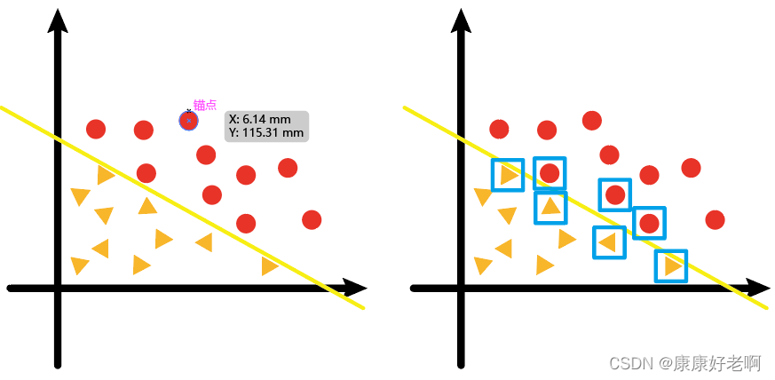
Concept: The sample points located near the classification hyperplane are called support vectors

In mathematics, the concept of a point is often replaced by a vector. For example, in the Cartesian coordinate system, the coordinates of point A are (3,4), we can think that it represents the vector OA = (3,4)

Now we have a two-dimensional sample point (vector) as shown in the left picture below, where the yellow line is the classification line calculated by linear regression; and those points close to the regression line in the right picture (marked with a blue square) are called support vector.

The meaning of "support" can be understood as follows:

​ Those points close to the classification boundary are the points that affect the direction of the regression line (hyperplane); points farther away from the classification boundary, they have no effect on how the regression line (hyperplane) is drawn

If we understand "machine" as "algorithm", then support vector machine is not difficult to understand as "algorithm related to support points (finding classification hyperplane)"

The following is a more standard concept of support vector machine:

Support Vector Machine (SVM)

It is a binary classification model, and its basic model is a linear classifier with the largest interval defined in the feature space.

For the following data sets, a regression line should be used to separate them. There are three lines ①, ②, and ③. Which one works best?

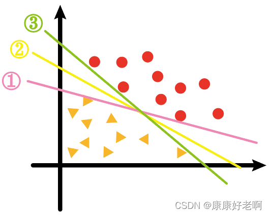
I think most people will think it is ②. Although the three lines are all satisfied to separate the triangle and the circle, for the ② line, the distance from the support vectors of the triangle and the circle to the ② line looks more "balanced", as if separating it from the middle.

In fact, the meaning of support vector machine refers to the algorithm that finds the sum of the distances from the support vector to the hyperplane as large as possible.

In fact, according to the basic inequality, the sum of the distances is the largest and the distance is more "balanced" is actually equivalent

Then here comes the concept of the maximum margin hyperplane

maximum margin hyperplane

The corresponding line ② in the figure above—that is, what we see as the most "balanced line" is actually a line that separates the two types of samples with the maximum interval (high-dimensional one is called a hyperplane), that is, the maximum interval hyperplane.

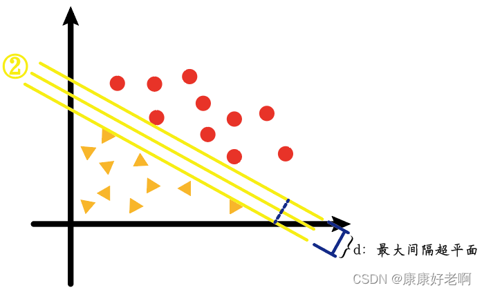
We will find that the sample interval of the two lines ① and ③ is much smaller than that of ②, as shown in the figure below

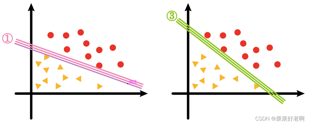
And what our support vector machine algorithm (SVM) essentially seeks is ② such a line, plane or hyperplane

Soft and hard intervals

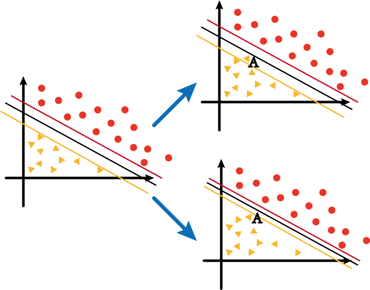
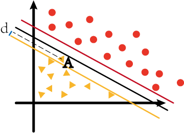
Assume that yellow, black and red in the coordinate system on the left in the above figure are negative/decision/positive hyperplanes respectively, and at this time if a new data point AA is added between the yellow line and the red $A$ , then whether to adjust around the hyperplane will be divided into two cases:

• The first is Figure 1 in the upper right corner, although AA is added$A$ , but still keep it between the yellow and red lines;
• The second is Figure 2 in the lower right corner, with $With\; the\; addition\; of\; A$ , the hyperplane also changes, and finally guarantees that$A$ is below the yellow line.

The distance between the yellow line and the red line in the first case is called soft interval; the distance between the yellow line and red line in the second case is called hard interval.

SVM optimization problem solving ideas

In linear algebra, any hyperplane can be described by the following linear equation:
$$W^{T}X+b=0$$
of which
$$W=[w_1,w_2,\cdot \cdot \cdot ，w_n]$$

$$X=[x_1,x_2,\cdot \cdot \cdot ，x_n]$$

is the coefficient matrix, after the matrix W is transposed

$$\left[\begin{array}{c}{W}_1\\ W_2\\ \cdot \\ \cdot \\ \cdot \\ W_n\end{array}\right]$$

$$

故
$$W^{T}X=w_1{x}_1+w_2{x}_2+w_3{x}_3+\cdot \cdot \cdot +w_n{x}_n$$
It is the hyperplane function expression we normally see

According to the distance formula from point to line

$$\frac{|Ax+By+C|}{\sqrt{A^2+B^2}}$$
Expand from two dimensions to high dimension∣
$$\frac{|w_1{x}_1+w_2{x}_2+w_3{x}_3+\cdot \cdot \cdot +w_n{x}_n+b|}{\sqrt{w_1^2+w_2^2+\cdot \cdot \cdot +w_n^2}}$$
其中
$$w_1{x}_1+w_2{x}_2+w_3{x}_3+\cdot \cdot \cdot +w_n{x}_n=W^{T}X$$
is the formula
$$\sqrt{w_1^2+w_2^2+\cdot \cdot \cdot +w_n^2}=||W||$$
is the definition of the modulus of the vector

For a two-dimensional vector X = (3,4), its modulus
$$||X||=\sqrt{3^2+4^2}=5$$
high-dimensional vectors and so on

So the above high-dimensional distance formula can be transformed into

$$\frac{|W^{T}X+b|}{||W||}$$

Mathematical Principles of Support Vector Machines

Through the above introduction, we have a general understanding of the function and simple principle of the support vector machine. Let's introduce the mathematical principle and algorithm of support vector machine in detail.

• Step 1: Establish the support vector equation

First of all, let me add the content of the hyperplane introduced above. We generally call the hyperplane used for separation in the middle as the decision hyperplane, and the decision hyperplane is also the hyperplane we finally obtain. There are two hyperplanes in the positive direction and negative direction of the decision hyperplane: a positive hyperplane and a negative hyperplane. These two hyperplanes are used to assist in generating decision hyperplanes. For simplicity, we only consider two-dimensional support vector machines.

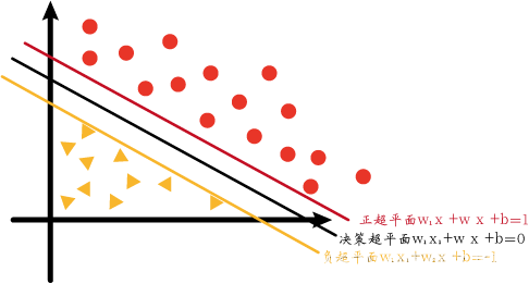
The equations of the positive hyperplane, decision hyperplane and negative hyperplane in the figure are as follows:
$$\begin{gathered} w_1{x}_1+w_2{x}_2+b=1 \\ {w}_1{x}_1+w_2{x}_2+b=0 \\ {w}_1{x}_1+w_2{x}_2+b=-1 \end{gathered}$$
is not the only way to write a hyperplane. In the previous basic part, we introduced how to express linear equations in matrices. This way of writing is just an equivalent variant (transposition) of the above, which is convenient for subsequent operations.

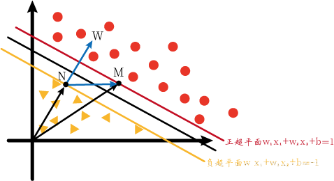
Now we assume that there are two support vectors M and N on the positive hyperplane and negative hyperplane respectively. They respectively satisfy the following formula:
$$\begin{gathered} w_1{x}_1+w_2{x}_2+b=1 \\ {w}_1{x}_{1n}+w_2{x}_2+b=-1 \end{gathered}$$
The two existing equations do not have any effect or inspiration for us. Considering that the common factors$w_1、w_2$, and have constant $b$ , so we take the difference between the two formulas and get the following result:
$$w_1(x_1-x_{1n})+w_2(x_2-x_2)=2$$
If we regard the above formula as a dot product of two vectors, we will get:
$$\vec{w}(\overrightarrow{x_m}-\overrightarrow{x_n})=2$$
in$\vec{w}=[w_1{w}_2]$，$\overrightarrow{x_m}=[x_1{x}_2{]}^T$，$\overrightarrow{x_n}=[x_{1n}{x}_2{]}^T$

Conditions $\vec{a}\cdot \vec{b}=||\vec{a}||\ast ||\vec{b}||\ast cos\theta$，
$$||\vec{w}||\ast ||\overrightarrow{x_m}-\overrightarrow{x_n}||\ast cos\theta =2$$
Among them$||\vec{w}||=\sqrt{w_1^2+w_2^2}$。

移题
$$||\overrightarrow{x_m}-\overrightarrow{x_n}||\ast cos\theta =\frac{2}{||\vec{w}||}$$

By transposing $x$ give$w$ are on the left and right sides of the equation. The coordinates of the data points are on the left, and the weight values ​​to be found are on the right.

• Step 2: Find the maximum interval $L$ expression

Here we might as well think about $||\overrightarrow{x_m}-\overrightarrow{x_n}||\ast The\; meaning\; of\; cos\theta$ .

So we draw the picture below and try to observe the meaning of the above formula from a geometric point of view.

We know that the vector dot product can be converted into a projection, that is, the modulus of a vector is multiplied by $Cos\theta$ is projected to the direction of another vector, and the same direction will greatly facilitate calculation.

So we draw the following coordinate system and vectors (referred to as Figure 1). We want to use vector dot product projection, but we don't know MN and $\vec{w}$angle.

But we can convert. We know that M and N are on the positive and negative hyperplanes, so what if M and N are on the decision hyperplane? Since the equations of these three hyperplanes are only different on the right side of the equal sign, if M and N are on the decision hyperplane, $\vec{w}$It should be the same as pictured above. So we might as well set M and N on the decision hyperplane first. We can draw the following graph (call it Figure 2):

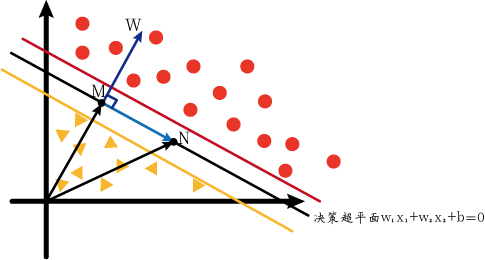
At this time, M and N respectively satisfy the following formula:
$$\begin{gathered} w_1{x}_1+w_2{x}_2+b=0 \\ {w}_1{x}_{1n}+w_2{x}_2+b=0 \end{gathered}$$
, we can get:
$$w_1(x_1-x_{1n})+w_2(x_2-x_2)=0$$
即
$$\vec{w}(\overrightarrow{x_m}-\overrightarrow{x_n})=$$
A dot product of$$0\; vectors\; is\; zero\; indicating\; that\; the\; two\; vectors\; are\; perpendicular\; to\; each\; other.$$Observe the above figure,$\overrightarrow{x_m}-\overrightarrow{x_n}$That is $\overrightarrow{NM}$. And this means that $\vec{w}$Perpendicular to the decision hyperplane, that is, perpendicular to the positive and negative hyperplanes. Well, at this time we turn back from Figure 2 to Figure 1, and we will release Figure 1 again for the convenience of explanation.

Since $\vec{w}$is perpendicular to the hyperplane, so $||\overrightarrow{NM}||$在$\vec{w}$The projection on is the maximum interval $L$ .$||\overrightarrow{NM}||=||\overrightarrow{x_m}-\overrightarrow{x_n}||\ast cos\theta$，故
$$L=\frac{2}{||\vec{w}||}$$

• Step 3: Find $L$ constraints, resulting in an optimization problem

Positive hyperplane: all red points belong to the positive class, so $y_i=1$ ; all red points are above the positive hyperplane, so$\vec{w}\cdot \overrightarrow{x_i}+b\ge 1$

Negative hyperplane: all yellow points belong to the negative class, so $y_i=-1$ ; all yellow points are below the negative hyperplane, so$\vec{w}\cdot \overrightarrow{x_i}+b\le 1$

The above two situations can be summarized into the following formula:
$$y_i\ast (\vec{w}\cdot \overrightarrow{x_i}+b)\ge 1$$
and this formula is the constraint condition.

Therefore, the problem of finding a decision hyperplane is transformed into:

在$y_i\ast (\vec{w}\cdot \overrightarrow{x_i}+b)\ge 1$ condition,$||\vec{w}||$ minimum value.

由于$||\vec{w}||=\sqrt{w_1^2+w_2^2}$contains a root sign, so the minimum value is not very easy to find. So let's convert it, will $||\vec{w}||$ is transformed into$\frac{||\vec{w}|{|}^2}{2}$, so the problem is equivalent to:

在$y_i\ast (\vec{w}\cdot \overrightarrow{x_i}+b)\ge 1$ condition,$\frac{||\vec{w}|{|}^2}{2}$minimum value.

• Step 4: Solve the first four conditions for the solution of the optimization problem

We will use the method of Lagrange multipliers to solve this kind of problem.

But there is a problem, that is, the constraint condition $y_i\ast (\vec{w}\cdot \overrightarrow{x_i}+b)\ge 1$ is an inequality rather than an equality, so we have to go through a step of conversion to convert the inequality into an equality.

We have $y_i\ast (\vec{w}\cdot \overrightarrow{x_i}+b)\ge 1$ Transform$y_i\ast (\vec{w}\cdot \overrightarrow{x_i}+b)-1=p_i^2$, since $p_i^2\ge 0$恒成立，故$y_i\ast (\vec{w}\cdot \overrightarrow{x_i}+b)-1\ge 0$ constant is established.

So the original problem is equivalent to:

在$y_i\ast (\vec{w}\cdot \overrightarrow{x_i}+b)-1=p_i^2$Under the condition, $\frac{||\vec{w}|{|}^2}{2}$minimum value.

Lower-surface structural Rager Rokuhi function:
$$L(w,b,l_i,p_i)=\frac{||\vec{w}|{|}^2}{2}-\sum _{i=1}^s{l}_i\ast (y_i\ast (\vec{w}\cdot \overrightarrow{x_i}+b)-1-p_i^2)$$
and then solve it. The Lagrange function takes the partial derivative for each unknown and sets it equal to zero.
$$\frac{\partial L}{\partial w}=0;\frac{\partial L}{\partial b}=0;\frac{\partial L}{\partial {\lambda }_i}=0;\frac{\partial L}{\partial p_i}=0$$
Let's calculate one by one below.

• First $\frac{\partial L}{\partial w}=0$。$w$ appears in two positions, namely$\frac{||\vec{w}|{|}^2}{2}$和${\sum }_{i=1}^s{l}_i\ast y_i\ast (\vec{w}\cdot \overrightarrow{x_i}+b)$ , it is easy to derive the following formula:

$$\vec{w}-\sum _{i=1}^s{l}_i{y}_i\overrightarrow{x_i}=0\cdot \cdot \cdot \cdot \cdot \cdot \cdot \cdot \cdot \cdot \cdot \cdot ①$$

• Then $\frac{\partial L}{\partial b}=0$。$b$ only appears in one position,${\sum }_{i=1}^s{l}_i\ast y_i\ast b$ , it is easy to derive the following formula:

$$\sum _{i=1}^s{l}_i{y}_i=0\cdot \cdot \cdot \cdot \cdot \cdot \cdot \cdot \cdot \cdot \cdot \cdot ②$$

• Then $\frac{\partial L}{\partial {\lambda }_i}=0。$ λ i$l_i$only appear in one position, as ${\sum }_{i=1}^s{l}_i\ast (y_i\ast (\vec{w}\cdot \overrightarrow{x_i}+b)-1-p_i^2)$ . Originally, the result of partial derivative should be${\sum }_{i=1}^s{y}_i\ast (\vec{w}\cdot \overrightarrow{x_i}+b)-1-p_i^2=0$ , but according to the constraints,$y_i\ast (\vec{w}\cdot \overrightarrow{x_i}+b)-1-p_i^2=0$ , there is no need to use the summation sign.

$$y_i\ast (\vec{w}\cdot \overrightarrow{x_i}+b)-1-p_i^2=0\cdot \cdot \cdot \cdot \cdot \cdot \cdot \cdot \cdot \cdot \cdot \cdot ③$$

• Finally $\frac{\partial L}{\partial p_i}=0$。$p_i$Appears in only one position, ${\sum }_{i=1}^s{l}_i\ast (-p_i^2)$ , it is easy to derive the following formula:

$$2{min}_i{p}_i=0\cdot \cdot \cdot \cdot \cdot \cdot \cdot \cdot \cdot \cdot \cdot \cdot ④$$

The following steps are to use ①~④ and the original formula to find $||\vec{w}||$ minimum value. First, we divide the left and right sides of equation ④ by 2 and multiply by$p_i$, the formula:
$$l_i{p}_i^2=0$$
is doing this because there is a$p_i^2$, which can simplify the calculation to some extent. We substitute formula ③ into formula ④ and get:
$$l_i(y_i\ast (\vec{w}\cdot \overrightarrow{x_i}+b)-1)=0$$
is very interesting. Before we got yi ∗ ( w ⃗ ⋅ xi ⃗ + b ) ≥ 1in the third step$y_i\ast (\vec{w}\cdot \overrightarrow{x_i}+b)\ge 1$ , the above formula can only be established in two situations:

① $y_i\ast (\vec{w}\cdot \overrightarrow{x_i}+b)-1)00$ ,$l_i=0$;

② $y_i\ast (\vec{w}\cdot \overrightarrow{x_i}+b)-1=0$ ,$l_i\ne 0$。

• Step 5: Obtain the fifth condition for the solution of the optimization problem

对于Ragerangi function $L(w,b,l_i,p_i)=\frac{||\vec{w}|{|}^2}{2}-{\sum }_{i=1}^s{l}_i\ast (y_i\ast (\vec{w}\cdot \overrightarrow{x_i}+b)-1-p_i^2)$ , when the constraints are not satisfied, that is,$$y_i\ast (\vec{w}\cdot \overrightarrow{x_i}+b)-1<0$$ , if$l_i<0$，则${\sum }_{i=1}^s{l}_i\ast (y_i\ast (\vec{w}\cdot \overrightarrow{x_i}+b)-1-p_i^2)>0$，而$L(w,b,l_i,p_i)$ will be smaller. According to the properties of the Lagrangian function, the value of the Lagrangian function is smaller if the constraints are met. This means that$l_i$It is unreasonable to be less than 0, so it should be greater than or equal to 0.

We can also explain this problem through images.

We assume that it is a two-dimensional space. In this two-dimensional space, the horizontal and vertical coordinates are $w_1$Sum $w_2$, N $||\vec{w}||=\sqrt{w_1^2+w_2^2}$The geometric meaning expressed on the image is a circle with the center as the origin, and the radius is $\sqrt{w_1^2+w_2^2}$circle.

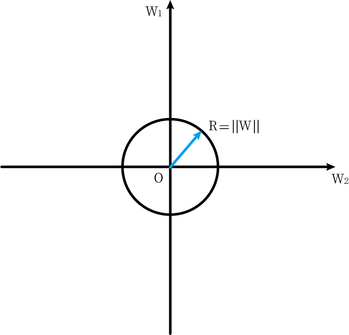
The optimization problem we require is $min\frac{||\vec{w}|{|}^2}{2}$, which is $||\vec{w}||$ It is obtained when the minimum value is taken. And since$||\vec{w}||$ is the radius of the circle, so we want the circle to be as small as possible.

Now we add constraints. The first constraint is $$g_1=y_1\ast (\vec{w}\cdot \overrightarrow{x_1}+b)-1\ge 0$$ , it means on the image that the feasible area is above a straight line (light green), as shown in the following figure:

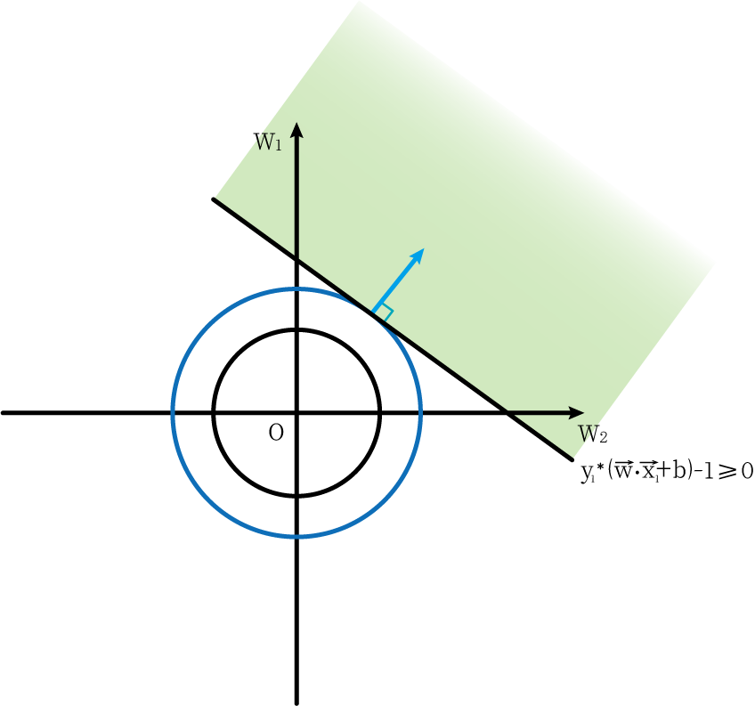
And the situation where a point on the circle can be within the feasible area and the radius of the circle is the smallest is that the circle is tangent to the line (indicated by the dark blue circle in the figure)

At this point we add another restriction, $$g_2=y_2\ast (\vec{w}\cdot \overrightarrow{x_2}+b)-1\ge 0$$ . At this time, under the two constraints, the smallest circle is the circle passing through the intersection of two straight lines. At this time$\vec{w}=(w_1,w_2)$ direction (represented by the red line) as long as it is within two straight lines.

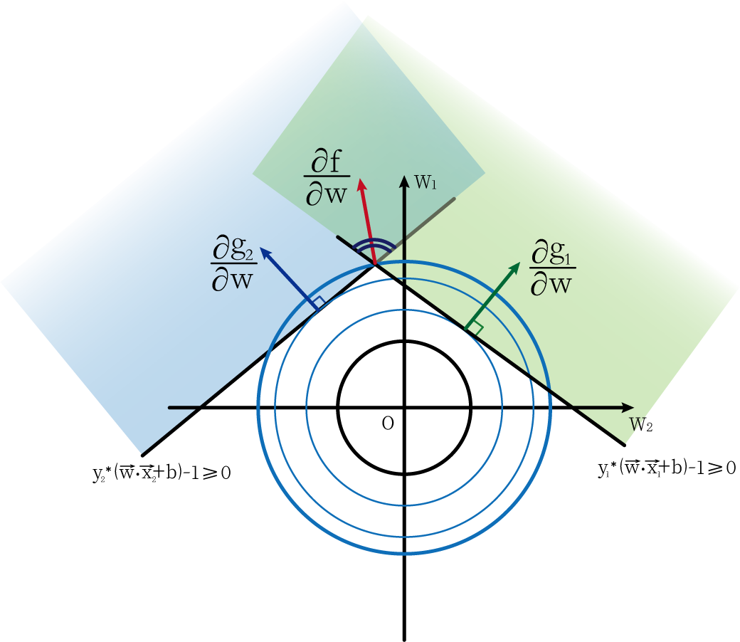
Through the intuitive understanding of the above figure, we can also get the following formula: Vector $\frac{\partial f}{\partial w}$Can be obtained by $\frac{\partial g_1}{\partial w}and\frac{\partial g_2}{\partial w}$Linear expression, and their coefficients $l_1$and $l_2$Both are non-negative numbers (understood intuitively or with vector triangles).
$$\frac{\partial f}{\partial w}=l_1\frac{\partial g_1}{\partial w}+l_2\frac{\partial g_2}{\partial w}$$
The above image can also help us understand, $l_i$Why is greater than or equal to 0. We also get the fifth condition:
$$l_i\ge 0\cdot \cdot \cdot \cdot \cdot \cdot \cdot \cdot \cdot \cdot \cdot \cdot ⑤$$
In summary, the above five conditions that we have reached and understood, or so-called KKT conditions:
$$\begin{gathered} \vec{w}-\sum _{i=1}^s{l}_i{y}_i\overrightarrow{x_i}=0\cdot \cdot \cdot \cdot \cdot \cdot \cdot \cdot \cdot \cdot \cdot \cdot \cdot \cdot \cdot \cdot \cdot \cdot \cdot \cdot ① \\ \sum _{i=1}^s{l}_i{y}_i=0\cdot \cdot \cdot \cdot \cdot \cdot \cdot \cdot \cdot \cdot \cdot \cdot \cdot \cdot \cdot \cdot \cdot \cdot \cdot \cdot \cdot \cdot \cdot \cdot \cdot ② \\ {y}_i\ast (\vec{w}\cdot \overrightarrow{x_i}+b)-1-p_i^2=0\cdot \cdot \cdot \cdot \cdot \cdot \cdot \cdot \cdot \cdot \cdot \cdot ③ \\ 2{min}_i{p}_i=0\cdot \cdot \cdot \cdot \cdot \cdot \cdot \cdot \cdot \cdot \cdot \cdot \cdot \cdot \cdot \cdot \cdot \cdot \cdot \cdot \cdot \cdot \cdot \cdot \cdot \cdot \cdot \cdot ④ \\ {l}_i\ge 0\cdot \cdot \cdot \cdot \cdot \cdot \cdot \cdot \cdot \cdot \cdot \cdot \cdot \cdot \cdot \cdot \cdot \cdot \cdot \cdot \cdot \cdot \cdot \cdot \cdot \cdot \cdot \cdot \cdot \cdot \cdot ⑤ \end{gathered}$$

• Step 6: Convert to SVM dual problem

The dual problem is a common method for solving linear programming problems. The difficulty of solving a problem can sometimes be greatly simplified by converting a problem into its dual.

Let's review the original question first:

在$g_i(w,b)=y_i\ast (\vec{w}\cdot \overrightarrow{x_i}+b)-1=p_i^2$condition, $beg\frac{||\vec{w}|{|}^2}{2}$minimum value.

Let's first assume that the optimal solution to the original problem is $w^{\ast }、b^{\ast }$。然后设
$$q({\lambda }_i)=min\left(L\right(w,b,l_i))=min(\frac{||\vec{w}|{|}^2}{2}-\sum _{i=1}^s{l}_i\ast (y_i\ast (\vec{w}\cdot \overrightarrow{x_i}+b)-1-p_i^2))$$
Substitution$w^{\ast }、b^{\ast }$ , possible-to-be-obtainable formula:
$$q({\lambda }_i)=min\left(L\right(w,b,l_i))\le min\left(L\right(w^{\ast },b^{\ast },l_i))$$
即$min(\frac{||\vec{w}|{|}^2}{2}-{\sum }_{i=1}^s{l}_i\ast (y_i\ast (\vec{w}\cdot \overrightarrow{x_i}+b)-1-p_i^2))\le \frac{||\overrightarrow{w^{\ast }}|{|}^2}{2}-{\sum }_{i=1}^s{l}_i\ast (y_i\ast (\overrightarrow{w^{\ast }}\cdot \overrightarrow{x_i}+b^{\ast })-1-p_i^2)$

The presence of a less than or equal sign is defined by $It\; is\; determined\; by\; the\; min$ minimum function.

∑ i = 1 s λ i ∗ ( yi ∗ ( w ∗ ⃗ ⋅ xi ⃗ + b ∗ ) − 1 − pi 2 ) \sum_{i=1}^s\lambda_i*( y_i ${\sum }_{i=1}^s{l}_i\ast (y_i\ast (\overrightarrow{w^{\ast }}\cdot \overrightarrow{x_i}+b^{\ast })-1-p_i^2)$必定 is greater than0，故
$$\frac{||\overrightarrow{w^{\ast }}|{|}^2}{2}-\sum _{i=1}^s{l}_i\ast (y_i\ast (\overrightarrow{w^{\ast }}\cdot \overrightarrow{x_i}+b^{\ast })-1-p_i^2)\le \frac{||\overrightarrow{w^{\ast }}|{|}^2}{2}$$
And because $\overrightarrow{w^{\ast }}$is the optimal solution to the original problem, so we can get:
$$\frac{||\overrightarrow{w^{\ast }}|{|}^2}{2}\le \frac{||\vec{w}|{|}^2}{2}$$
So we can get the following inequality chain:
$$q({\lambda }_i)\le min\left(L\right(w^{\ast },b^{\ast },l_i))\le \frac{||\overrightarrow{w^{\ast }}|{|}^2}{2}\le \frac{||\vec{w}|{|}^2}{2}$$
We assume that $l_i^{\ast }isq\left({\lambda }_i\right)$ is the optimal solution.∪q
$$q\left({\lambda }_i\right)\le q\left({\lambda }_i^{\ast }\right)\le \frac{||\overrightarrow{w^{\ast }}|{|}^2}{2}\le \frac{||\vec{w}|{|}^2}{2}$$
Well, at this point we can transform the original problem into a dual problem.

Original question:

• 在$g_i(w,b)=y_i\ast (\vec{w}\cdot \overrightarrow{x_i}+b)-1\ge$Under the condition of$0$$beg\frac{||\vec{w}|{|}^2}{2}$minimum value.

Dual problem:

• 在$l_i\ge 0$的条件下，求$q({\lambda }_i)=min\left(L\right(w,b,l_i))$ maximum value.

当$q\left({\lambda }_i^{\ast }\right)=\frac{||\overrightarrow{w^{\ast }}|{|}^2}{2}$When , the two problems are strong dual problems, and the optimal solution should be obtained at the same time. The proof is as follows:

Since
$$q\left({\lambda }_i\right)\le \frac{||\vec{w}|{|}^2}{2}$$
So
$$q\left({\lambda }_i^{\ast }\right)\le \frac{||\vec{w}|{|}^2}{2}$$
故
$$\frac{||\overrightarrow{w^{\ast }}|{|}^2}{2}\le \frac{||\vec{w}|{|}^2}{2}$$
And according to the previous $q({\lambda }_i)\le min\left(L\right(w^{\ast },b^{\ast },l_i))\le \frac{||\overrightarrow{w^{\ast }}|{|}^2}{2}$,Let
$$q\left({\lambda }_i\right)\le \frac{||\overrightarrow{w^{\ast }}|{|}^2}{2}=q\left({\lambda }_i^{\ast }\right)$$
so$q({\lambda }_i^{\ast })$为$q\left({\lambda }_i\right)$ maximum solution.

Therefore, it is proved that under the condition of strong duality, the optimal solutions of the primal problem and the dual problem are obtained at the same time.

• Step 7: Optimizing the Equation

According to the previous Lagrange function, we have obtained:
$$max(q(\lambda ))=max(min(\frac{||\vec{w}||}{2})-\sum _{i=1}^s{l}_i\ast (y_i\ast (\overrightarrow{w^{\ast }}\cdot \overrightarrow{x_i}+b^{\ast })-1)))$$
将KKT condition代入化简可得：
$$max\left(q\right(\lambda ))=max(\sum _{i=1}^s{l}_i-\frac{1}{2}\sum _{i=1}^s\sum _{j=1}^s{l}_i{l}_j{y}_i{y}_j\overrightarrow{x_i}\cdot \overrightarrow{x_j})$$

• Step 8: Deriving the Algorithm Steps

Above we derived the following formula:

① $y_i\ast (\vec{w}\cdot \overrightarrow{x_i}+b)-1>0$ ,$l_i=0$;

② $y_i\ast (\vec{w}\cdot \overrightarrow{x_i}+b)-1=0$ ,$l_i\ne 0$。

At the same time, we also deduce that $l_i\ge 0$ for this condition.

According to the above two conditions we can draw some conclusions.

• If the data points are in the positive and negative hyperplane $\vec{w}\cdot \overrightarrow{x_i}+b\pm 1=0$ , because$|y_i|=1$，所以$y_i\ast (\vec{w}\cdot \overrightarrow{x_i}+b)-1=0$ , it belongs to the case ②, so$l_i＞0$。

• If the data point is not on the positive and negative hyperplane $\vec{w}\cdot \overrightarrow{x_i}+b\pm 1=0$ , it belongs to the case ①, so$l_i=0$ . Then$l_i=0$ Substitutable$l_i(y_i\ast (\vec{w}\cdot \overrightarrow{x_i}+b)-1)=0$。

The above derivation shows that we are calculating the hyperplane weight value $When\; w$ only needs to use support vectors (data points on the positive and negative hyperplanes), no non-support vectors are required.

With the previous foreshadowing, we can get the support vector machine SVM algorithm.

① Obtain $l_i$valuemax
$$\begin{gathered} max(q(\lambda ))=max(\sum _{i=1}^s{l}_i-\frac{1}{2}\sum _{i=1}^s\sum _{j=1}^s{l}_i{l}_j{y}_i{y}_j\overrightarrow{x_i}\cdot \overrightarrow{x_j}) \\ where{\lambda }_i\ge 0 \end{gathered}$$
② Underlying KKT condition
$$\vec{w}=\sum _{i=1}^s{l}_i{y}_i\overrightarrow{x_i}$$
can find $\vec{w}$

title

③ 根据$y_i\ast (\vec{w}\cdot \overrightarrow{x_i}+b)-1=0$ solves for$b$

Dimension Ascension Transformation and Kernel Techniques

Let's look at the following scenario:

For example, now there are some data points on the 1D x-axis, red and blue. We now want to use a function (a constant for one dimension) to divide the red and blue points. It can be seen intuitively that this is impossible.

However, if the above picture is produced by projecting a two-dimensional plane figure onto the one-dimensional x-axis, we may find a different world if we "restore" the two-dimensional plane:

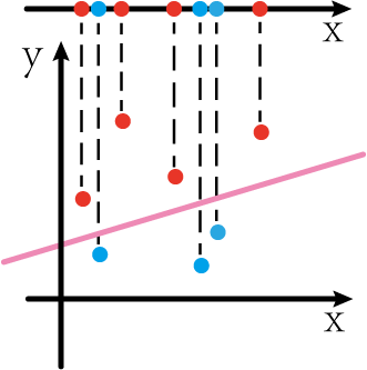
As shown above, if we can convert one-dimensional data points into two-dimensional data points by some methods, then we seem to be able to easily divide the data points (the pink line in the figure)

This process is known as dimension-up conversion.

We can also use this method in support vector machines. Let's review the optimization equation first:
$$\begin{gathered} max(q({\lambda }_i))=max(\sum _{i=1}^s{l}_i-\frac{1}{2}\sum _{i=1}^s\sum _{j=1}^s{l}_i{l}_j{y}_i{y}_j\overrightarrow{x_i}\cdot \overrightarrow{x_j}) \\ where{\lambda }_i\ge 0 \end{gathered}$$
$\overrightarrow{x_i}\cdot \overrightarrow{x_j}$Indicates the dot product of the corresponding vector coordinates in the original dimension. But in fact, the above equation is unsolvable, so we can use the kernel technique to perform dimension-boosting transformation. We will pass a function $T\left(x\right)$ performs a dimension-boosting transformation operation, and this function is called a dimension conversion function. Through the dimension conversion function, the original$\overrightarrow{x_i}$becomes $T(\overrightarrow{x_i})$，$\overrightarrow{x_j}$becomes $T\left(\overrightarrow{x_j}\right)$ . So the original problem is transformed into the following formula:
$$\begin{gathered} max(q({\lambda }_i))=max(\sum _{i=1}^s{l}_i-\frac{1}{2}\sum _{i=1}^s\sum _{j=1}^s{l}_i{l}_j{y}_i{y}_{j}T(\overrightarrow{x_i})\cdot T(\overrightarrow{x_j})) \\ where{\lambda }_i\ge 0 \end{gathered}$$
In fact, here we can pass$\overrightarrow{x_i}、\overrightarrow{x_j}$写出$T(\overrightarrow{x_i})、T(\overrightarrow{x_j})$ , and then perform the dot product operation, or directly set$K(\overrightarrow{x_i},\overrightarrow{x_j})=T(\overrightarrow{x_i})\cdot T\left(\overrightarrow{x_j}\right)$ , and then calculate. The difference between the two is that the latter is directly$\overrightarrow{x_i}\cdot \overrightarrow{x_j}$It is regarded as an unknown number and substituted into the calculation as a whole. And here $K(\overrightarrow{x_i},\overrightarrow{x_j})$ is the kernel function. Its general expression is as follows:
$$K(\overrightarrow{x_i},\overrightarrow{x_j})=(c+\overrightarrow{x_i}\cdot \overrightarrow{x_j}{)}^d$$
then parameters$What\; is\; the\; role\; of\; candd$ ?

for the same $d$ , different$For\; c$ ,$c$ can control the presence or absence of low-order terms and the coefficient of low-order terms;

for the same $c$ , differentddFor$d$$The\; size\; of\; d$ determines the highest dimension size.

In addition, the kernel function can also be formed by a linear combination of multiple kernel functions, such as: $K_1^{\prime }(\overrightarrow{x_i},\overrightarrow{x_j})+K_2^{\prime }(\overrightarrow{x_i},\overrightarrow{x_j})$

There is also a special kernel function that converts two dimensions into infinite dimensions. This kernel function is a Gaussian kernel function (RBF), and its formula is as follows:
$$K(\overrightarrow{x_i},\overrightarrow{x_j})=e^{-\gamma ||\overrightarrow{x_i}-\overrightarrow{x_j}|{|}^2}$$

soft interval

The concept of soft and hard intervals has been explained in the previous article, and we will discuss them in detail below.

As shown in the figure above, there is a point A that violates the constraints and is within the yellow and black lines.

We know that the hard margin constraints are $y_i\ast (\overrightarrow{w^{\ast }}\cdot \overrightarrow{x_i}+b^{\ast })-1\ge 0$ . If point A violates the constraints, then point A satisfies the formula$y_a\ast (\overrightarrow{w^{\ast }}\cdot \overrightarrow{x_a}+b^{\ast })-1<0$ . We want to convert inequality into equality, we need a${ϵ}_a$To measure the error, the formula is as follows:
$${ϵ}_a=1-y_a\ast (\overrightarrow{w^{\ast }}\cdot \overrightarrow{x_a}+b^{\ast })$$
So the soft margin optimization problem is as follows:

在$g_i(w,b)=y_i\ast (\vec{w}\cdot \overrightarrow{x_i}+b)-1＞0$和$max(0,1-y_a\ast (\overrightarrow{w^{\ast }}\cdot \overrightarrow{x_a}+b^{\ast }))$condition,

$beg\frac{||\vec{w}|{|}^2}{2}+C{\sum }_{i=1}^s{ϵ}_i$minimum value.

We can compare with the previous hard-margin optimization problem:

在$g_i(w,b)=y_i\ast (\vec{w}\cdot \overrightarrow{x_i}+b)-Under\; the\; condition\; of\; 1>0$ ,

$beg\frac{||\vec{w}|{|}^2}{2}$minimum value.

In fact, the biggest difference between the soft interval and the hard interval is that there is one more term
$$C\sum _{i=1}^s{ϵ}_i$$
The meaning of this item is that all errors ${\sum }_{i=1}^s{ϵ}_i$Considering the optimization problem, this can also reduce the error when finding the minimum value. while the constant $C$ is artificially stipulated by us, and it plays a role in adjusting the tolerance of errors.

• $The\; larger\; C$ , it means that for${ϵ}_i$The smaller the tolerance, that is, the fewer errors in the final calculated results;
• $The\; smaller\; C$ is, it means that for${ϵ}_i$The greater the tolerance, that is, the greater the error in the final calculated result;