Kaggle's Time Series course code

Linear Regression With Time Series

This series records the number of hardcover books sold in a retail store in a 30-day period. Note that we have a column of hardcover observations with time-indexed dates.

import pandas as pd
df = pd.read_csv("../input/ts-course-data/book_sales.csv",
               index_col="Date",#指定某列为行索引，否则自动索引0, 1, .....
               parse_dates=["Date"],#parse_dates=[0,1,2,3,4] : 尝试解析0，1，2，3，4列为时间格式；
               ).drop("Paperback", axis=1)#删除列
df.head()#df.head(n):该方法用于查看dataframe数据表中开头n行的数据，若参数n未设置，即df.head()，则默认查看dataframe中前5行的数据。

Time step features are features that we can derive directly from the time index. The most basic time step feature is the time dummy variable, which counts the time steps in the sequence from beginning to end.

import numpy as np

df['Time'] = np.arange(len(df.index))#函数返回一个有终点和起点的固定步长的排列，如[1,2,3,4,5]，起点是1，终点是6，步长为1。

df.head()

The time dummy variable then lets us fit a curve to the time series in a time plot, where time forms the x-axis.

import matplotlib.pyplot as plt
import seaborn as sns
plt.style.use("seaborn-whitegrid")
plt.rc(
    "figure",
    autolayout=True,
    figsize=(11, 4),
    titlesize=18,
    titleweight='bold',
)
plt.rc(
    "axes",
    labelweight="bold",
    labelsize="large",
    titleweight="bold",
    titlesize=16,
    titlepad=10,
)
%config InlineBackend.figure_format = 'retina'#避免绘制模糊图像,JuypterNotebook中的默认绘图看起来有些模糊。

fig, ax = plt.subplots()
ax.plot('Time', 'Hardcover', data=df, color='0.75')
ax = sns.regplot(x='Time', y='Hardcover', data=df, ci=None, scatter_kws=dict(color='0.25'))
ax.set_title('Time Plot of Hardcover Sales');

To make lagged features, we shift the observations of the target series so that they appear to occur at a later time. Here we create a 1-step lag function, although multi-step moves are also possible.

df['Lag_1'] = df['Hardcover'].shift(1)#Pandas dataframe.shift()函数根据需要的周期数移动索引，并带有可选的时间频率。该函数采用称为周期的标量参数，该参数表示要在所需轴上进行的平移次数。
df = df.reindex(columns=['Hardcover', 'Lag_1'])#reindex重新构建索引

df.head()

Thus, the lag feature allows us to fit a curve to a lag plot, where each observation in the series corresponds to the previous observation.

fig, ax = plt.subplots()
ax = sns.regplot(x='Lag_1', y='Hardcover', data=df, ci=None,                 
                 scatter_kws=dict(color='0.25'))#sns.regplot()：绘图数据和线性回归模型拟合，ci置信区间，一般为None
ax.set_aspect('equal')#设置图形的宽高比，equal为1:1 
ax.set_title('Lag Plot of Hardcover Sales');

You can see from the lag plot that sales on a certain day (hardcover) are related to sales on the previous day (Lag_1). When you see a relationship like this, you know a delay function can be useful.

More generally, lag functions allow you to model serial dependencies. A time series has serial dependence when observations can be predicted from previous observations. In hardcover sales, we can predict that high sales one day will usually mean high sales the next day.

Adapting machine learning algorithms to time series problems is mostly about feature engineering with time indices and lags.

Example - Tunnel Traffic

Tunnel Traffic is a time series describing the number of vehicles passing through the Barreg Tunnel in Switzerland on a daily basis from November 2003 to November 2005. In this example, we will practice applying linear regression to time-stepped and lagged features.

from pathlib import Path
from warnings import simplefilter

import matplotlib.pyplot as plt
import numpy as np
import pandas as pd

simplefilter("ignore")  # ignore warnings to clean up output cells

# Set Matplotlib defaults
plt.style.use("seaborn-whitegrid")
plt.rc("figure", autolayout=True, figsize=(11, 4))
plt.rc(
    "axes",
    labelweight="bold",
    labelsize="large",
    titleweight="bold",
    titlesize=14,
    titlepad=10,
)
plot_params = dict(
    color="0.75",
    style=".-",
    markeredgecolor="0.25",
    markerfacecolor="0.25",
    legend=False,
)
%config InlineBackend.figure_format = 'retina'


# Load Tunnel Traffic dataset
data_dir = Path("../input/ts-course-data")
tunnel = pd.read_csv(data_dir / "tunnel.csv", parse_dates=["Day"])

# Create a time series in Pandas by setting the index to a date
# column. We parsed "Day" as a date type by using `parse_dates` when
# loading the data.
tunnel = tunnel.set_index("Day")

# By default, Pandas creates a `DatetimeIndex` with dtype `Timestamp`
# (equivalent to `np.datetime64`, representing a time series as a
# sequence of measurements taken at single moments. A `PeriodIndex`,
# on the other hand, represents a time series as a sequence of
# quantities accumulated over periods of time. Periods are often
# easier to work with, so that's what we'll use in this course.
tunnel = tunnel.to_period()

tunnel.head()

Exercise: Linear Regression With Time Series

# Setup feedback system
from learntools.core import binder
binder.bind(globals())
from learntools.time_series.ex1 import *

# Setup notebook
from pathlib import Path
from learntools.time_series.style import *  # plot style settings

import pandas as pd
import matplotlib.pyplot as plt
import numpy as np
import seaborn as sns
from sklearn.linear_model import LinearRegression


data_dir = Path('../input/ts-course-data/')
comp_dir = Path('../input/store-sales-time-series-forecasting')

book_sales = pd.read_csv(
    data_dir / 'book_sales.csv',
    index_col='Date',
    parse_dates=['Date'],
).drop('Paperback', axis=1)
book_sales['Time'] = np.arange(len(book_sales.index))
book_sales['Lag_1'] = book_sales['Hardcover'].shift(1)
book_sales = book_sales.reindex(columns=['Hardcover', 'Time', 'Lag_1'])

ar = pd.read_csv(data_dir / 'ar.csv')

dtype = {
    'store_nbr': 'category',
    'family': 'category',
    'sales': 'float32',
    'onpromotion': 'uint64',
}
store_sales = pd.read_csv(
    comp_dir / 'train.csv',
    dtype=dtype,
    parse_dates=['date'],
    infer_datetime_format=True,
)
store_sales = store_sales.set_index('date').to_period('D')
store_sales = store_sales.set_index(['store_nbr', 'family'], append=True)
average_sales = store_sales.groupby('date').mean()['sales']

One advantage of linear regression over more complex algorithms is that the models it creates are interpretable, making it easy to explain the contribution of each feature to the prediction. In the model target = weight * feature + bias, the weight tells you the average change in target per unit of change in the feature 

fig, ax = plt.subplots()
ax.plot('Time', 'Hardcover', data=book_sales, color='0.75')
ax = sns.regplot(x='Time', y='Hardcover', data=book_sales, ci=None, scatter_kws=dict(color='0.25'))
ax.set_title('Time Plot of Hardcover Sales');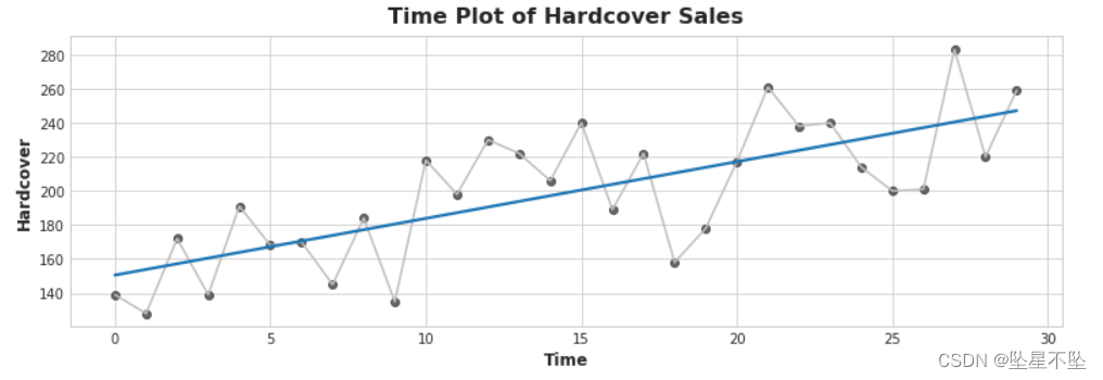

1) Interpret linear regression using time dummy variable 

The equation for the linear regression line is (approximately) hardcover = 3.33 * time + 150.5. How much do you expect the average hardcover book sales to change over 6 days? After you think about it, run the next cell

# View the solution (Run this line to receive credit!)
q_1.check()

A change in time of 6 steps corresponds to an average change in hardcover book sales of 6 * 3.33 = 19.98.

# Uncomment the next line for a hint
#q_1.hint()

Interpreting regression coefficients can help us identify serial dependencies in time plots. Consider model target = weight * lag_1 + error, where error is random noise and weight is a number between -1 and 1. In this case, the weight tells you how likely it is that the next time step will have the same sign as the previous time step, a weight close to 1 means the target is likely to have the same sign as the previous step, and a weight close to -1 means Goals may have opposite signs.

2) Interpreting linear regression with lagged features

fig, (ax1, ax2) = plt.subplots(2, 1, figsize=(11, 5.5), sharex=True)
ax1.plot(ar['ar1'])
ax1.set_title('Series 1')
ax2.plot(ar['ar2'])
ax2.set_title('Series 2');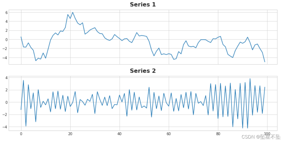

One of the series has the equation target = 0.95 * lag_1 + error and the other has the equation target = -0.95 * lag_1 + error, differing only in sign on the lag feature. Can you name the equations for each series?

# View the solution (Run this cell to receive credit!)
q_2.check()

# Uncomment the next line for a hint
#q_2.hint()

Now we will start competing data using Store Sales - Time Series Forecasting. The entire dataset contains nearly 1800 collections recording store sales across various product lines from 2013 to 2017. In this lesson, we will only be dealing with a single series (average_sales) that averages sales per day.

3) Fitting time step characteristics

Complete the code below to create a linear regression model that features a series of time steps of average product sales. Goals are in a column named "Sales".

from sklearn.linear_model import LinearRegression

df = average_sales.to_frame()

# YOUR CODE HERE: Create a time dummy
time = ____

df['time'] = time 

# YOUR CODE HERE: Create training data
X = ____  # features
y = ____  # target

# Train the model
model = LinearRegression()
model.fit(X, y)

# Store the fitted values as a time series with the same time index as
# the training data
y_pred = pd.Series(model.predict(X), index=X.index)


# Check your answer
q_3.check()

# Lines below will give you a hint or solution code
#q_3.hint()
#q_3.solution()

 

ax = y.plot(**plot_params, alpha=0.5)
ax = y_pred.plot(ax=ax, linewidth=3)
ax.set_title('Time Plot of Total Store Sales');