%matplotlib inline
import pandas as pd
import numpy as np

import matplotlib.pyplot as plt
import seaborn as sns
plt.rc('font', family='SimHei', size=13)

import os,gc,re,warnings,sys
warnings.filterwarnings("ignore")

path = '新建文件夹/推荐系统/零基础入门推荐系统 - 新闻推荐/'

# trn_click = pd.read_csv(path + 'train_click_log.csv')
trn_click = pd.read_csv(path+'train_click_log.csv',encoding= 'utf-8-sig',sep = r'\s*,\s*',header = 0)
trn_click.head()

item_df = trn_click = pd.read_csv(path + 'articles.csv',encoding= 'utf-8-sig',sep = r'\s*,\s*',header = 0)
item_df = item_df.rename(columns={'article_id': 'click_article_id'})  #重命名，方便后续match
item_df.head()

item_emb_df = pd.read_csv(path+'articles_emb.csv',encoding= 'utf-8-sig',sep = r'\s*,\s*',header = 0)
item_emb_df.head()

print(trn_click.columns.tolist())

Pandas Tutorial | Super easy-to-use Groupby usage explanation

# 对每个用户的点击时间戳进行排序
trn_click['rank'] = trn_click.groupby(['user_id'])['click_timestamp'].rank(ascending=False).astype(int)
tst_click['rank'] = tst_click.groupby(['user_id'])['click_timestamp'].rank(ascending=False).astype(int)


#计算用户点击文章的次数，并添加新的一列count
trn_click['click_cnts'] = trn_click.groupby(['user_id'])['click_timestamp'].transform('count')
tst_click['click_cnts'] = tst_click.groupby(['user_id'])['click_timestamp'].transform('count')

2. Data viewing

2.1, training set user click log

Merge trn_click and item_df into user click log-training set

#用户点击日志-训练集
trn_click = trn_click.merge(item_df, how='left', on=['click_article_id'])
trn_click.head()

trn_click.describe().T
trn_click.info()

<class 'pandas.core.frame.DataFrame'>
Int64Index: 1112623 entries, 0 to 1112622
Data columns (total 14 columns):
 #   Column               Non-Null Count    Dtype
---  ------               --------------    -----
 0   user_id              1112623 non-null  int64
 1   click_article_id     1112623 non-null  int64
 2   click_timestamp      1112623 non-null  int64
 3   click_environment    1112623 non-null  int64
 4   click_deviceGroup    1112623 non-null  int64
 5   click_os             1112623 non-null  int64
 6   click_country        1112623 non-null  int64
 7   click_region         1112623 non-null  int64
 8   click_referrer_type  1112623 non-null  int64
 9   rank                 1112623 non-null  int32
 10  click_cnts           1112623 non-null  int64
 11  category_id          1112623 non-null  int64
 12  created_at_ts        1112623 non-null  int64
 13  words_count          1112623 non-null  int64
dtypes: int32(1), int64(13)
memory usage: 123.1 MB

Total 20000 users

trn_click.user_id.nunique()#200000

Each user clicked on at least two articles in the training set

trn_click.groupby('user_id')['click_article_id'].count().min()  # 训练集里面每个用户至少点击了两篇文章

The click environment click_environment changes very stably, only 2102 times (accounting for 0.19%) the click environment is 1; only 25894 times (accounting for 2.3%) the click environment is 2;

trn_click['click_environment'].value_counts()

4    1084627
2      25894
1       2102
Name: click_environment, dtype: int64

Click the device group click_deviceGroup, device 1 accounts for the majority (61%), and device 3 accounts for 36%.

trn_click['click_deviceGroup'].value_counts()

1    678187
3    395558
4     38731
5       141
2         6
Name: click_deviceGroup, dtype: int64

2.2, test set user click log

#测试集用户点击日志
tst_click = tst_click.merge(item_df, how='left', on=['click_article_id'])
tst_click.head()

tst_click.describe()

tst_click.user_id.nunique()#50000

tst_click.groupby('user_id')['click_article_id'].count().min() # 注意测试集里面有只点击过一次文章的用户

The user IDs of the training set range from 0 to 199999, while the user IDs of the test set A range from 200000 to 249999.

During training, the data of the test set also needs to be included, which is called the full amount of data.

2.3. News article information data table

item_df.head().append(item_df.tail())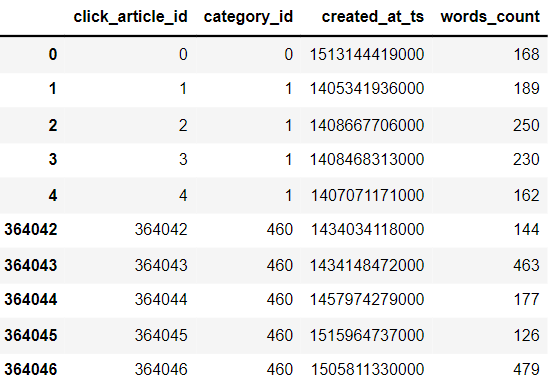

item_df.shape       # 364047篇文章

news word count

#新闻字数统计
item_df['words_count'].value_counts()

news category

#新闻类别
item_df['category_id'].nunique()#461
item_df['category_id'].hist()

2.4. News article embedding vector representation

item_emb_df.head()
item_emb_df.shape

3. Data Analysis

Merge user logs for training and testing sets

user_click_merge = trn_click.append(tst_click)

3.1. Number of times users repeatedly click news

#reset_index()重置索引。
user_click_count = user_click_merge.groupby(['user_id', 'click_article_id'])['click_timestamp'].agg({'count'}).reset_index()
user_click_count[:10]

	user_id	click_article_id	count
0	0	30760	1
1	0	157507	1
2	1	63746	1
3	1	289197	1
4	2	36162	1
5	2	168401	1
6	3	36162	1
7	3	50644	1
8	4	39894	1
9	4	42567	1

user_click_count[user_click_count['count']>7]


user_click_count['count'].unique()
#array([ 1,  2,  4,  3,  6,  5, 10,  7, 13], dtype=int64)

	user_id	click_article_id	count
311242	86295	74254	10
311243	86295	76268	10
393761	103237	205948	10
393763	103237	235689	10
576902	134850	69463	13

#用户重复点击新闻次数
user_click_count.loc[:,'count'].value_counts() #取count列所有行，统计不同的count出现的次数
#可以看出：有1605541（约占99.2%）的用户未重复阅读过文章，仅有极少数用户重复点击过某篇文章。 这个也可以单独制作成特征

1     1605541
2       11621
3         422
4          77
5          26
6          12
10          4
7           3
13          1
Name: count, dtype: int64

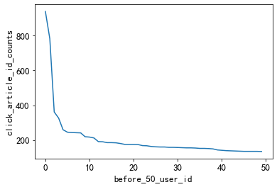
3.2. Distribution of users with different numbers of news clicks

3.2.1. Active users

The top 50 users with clicks all have more than 100 clicks. It is possible to define users whose clicks are greater than or equal to 100 times as active users.
This is a simple processing idea. To judge user activity, it is more comprehensive to combine click time.
Later, we will base it on the number of clicks and click time. to determine user activity.

#用户点击次数分析
user_click_item_count = sorted(user_click_merge.groupby('user_id')['click_article_id'].count(), reverse=True)
plt.plot(user_click_item_count)
plt.xlabel('user_id')
plt.ylabel('click_article_id_counts')

#点击次数在前50的用户
plt.plot(user_click_item_count[:50])
plt.xlabel('before_50_user_id')
plt.ylabel('click_article_id_counts')

3.2.2. Inactive users

There are a lot of users with less than or equal to two clicks, and these users can be considered as inactive users

#点击次数排名在[25000:50000]之间
plt.plot(user_click_item_count[25000:50000])

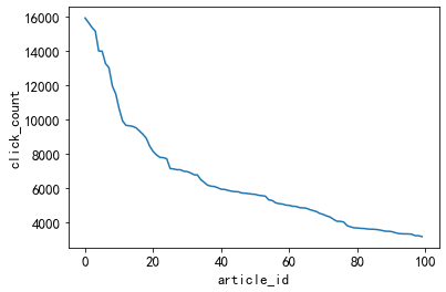
3.3. The number of news clicks

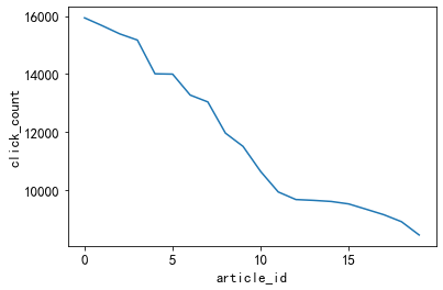
3.3.1 Hot news

'''The top 20 news articles with the most clicks, the number of clicks is greater than 2500.
Idea: These news can be defined as hot news, which is also a simple way to deal with it.
Later, we will also divide the popularity of articles according to the number of clicks and time. '''

item_click_count = sorted(user_click_merge.groupby('click_article_id')['user_id'].count(), reverse=True)
plt.plot(item_click_count)
plt.xlabel('article_id')
plt.ylabel('click_count')

plt.plot(item_click_count[:100])
plt.xlabel('article_id')
plt.ylabel('click_count')
#点击率排名前100的新闻点击量都超过1000次

plt.plot(item_click_count[:20])
plt.xlabel('article_id')
plt.ylabel('click_count')

3.3.2. Unpopular news

A lot of news is only clicked once or twice. Idea: It can be defined that these news are unpopular news

 plt.plot(item_click_count[3500:])

3.4. News co-occurrence frequency: the number of times two news articles appear consecutively

tmp = user_click_merge.sort_values('click_timestamp')
tmp['next_item'] = tmp.groupby(['user_id'])['click_article_id'].transform(lambda x:x.shift(-1))
union_item = tmp.groupby(['click_article_id','next_item'])['click_timestamp'].agg({'count'}).reset_index().sort_values('count', ascending=False)
union_item[['count']].describe()

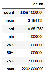
The average number of co-occurrences is 3.18, and the highest is 2202. The probability of two news articles appearing consecutively is high, indicating that the news users read are highly correlated.

x = union_item['click_article_id']
y = union_item['count']
plt.scatter(x, y)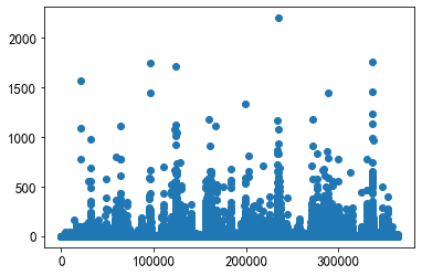

About 75,000 pairs co-occur at least once

plt.plot(union_item['count'].values[40000:])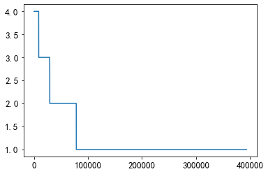

3.5. News article information

3.5.1. Times of appearance of different types of news

Less than 50 different types of news have a higher number of occurrences

#不同类型的新闻出现的次数
plt.plot(user_click_merge['category_id'].value_counts().values)
plt.xlabel('article_id')
plt.ylabel('appear_counts')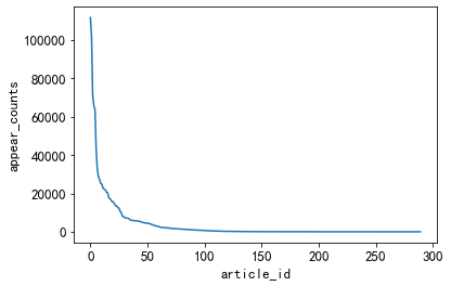

news with fewer occurrences

#出现次数比较少的新闻类型, 有些新闻类型，基本上就出现过几次
plt.plot(user_click_merge['category_id'].value_counts().values[150:])
plt.xlabel('article_id')
plt.ylabel('appear_counts')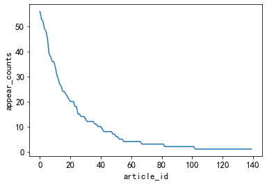

3.5.2. Number of news words

#新闻字数的描述性统计
user_click_merge['words_count'].describe()

plt.plot(user_click_merge['words_count'].values)

3.5.3. The preference of news types clicked by users

This feature can be used to measure whether the user's interests are extensive.

#用户偏好的新闻广泛程度
plt.plot(sorted(user_click_merge.groupby('user_id')['category_id'].nunique(), reverse=True))
plt.xlabel('user_id')
plt.ylabel('category_id')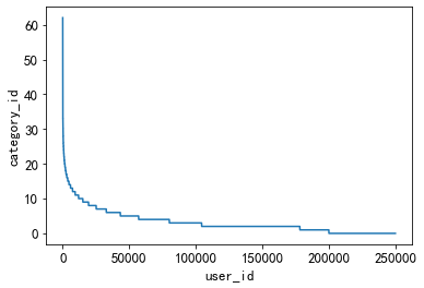

It can be seen from the figure that there are fewer users with a wide range of preference types, and most users have fewer preference types, less than 20 types.

3.5.4. Distribution of length of articles viewed by users

By counting the average word count of news clicked by different users, this can reflect whether users are more interested in long articles or short articles.

plt.plot(sorted(user_click_merge.groupby('user_id')['words_count'].mean(),reverse = True))
plt.xlabel('user_id')
plt.ylabel('avg_words_count')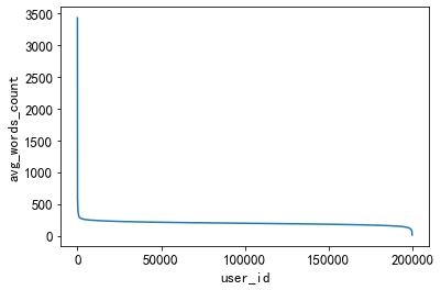

The average word count of articles read by a small group of people is very high, and the average number of words read by a small group of people is very low.

Most people prefer to read news between 200-400 words.

plt.plot(sorted(user_click_merge.groupby('user_id')['words_count'].mean(),reverse = True)[1000:45000])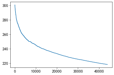

In the range of most people, people prefer to read news with a word count of 220-250 words.

3.6. Time Analysis of Users Clicking News


#为了更好的可视化，这里把时间进行归一化操作
from sklearn.preprocessing import MinMaxScaler
mm = MinMaxScaler()
user_click_merge['click_timestamp'] = mm.fit_transform(user_click_merge[['click_timestamp']])
user_click_merge['created_at_ts'] = mm.fit_transform(user_click_merge[['created_at_ts']])

user_click_merge = user_click_merge.sort_values('click_timestamp')

3.6.1. The average value of click time difference

Usage of shift(1) in pandas

def mean_diff_time_func(df, col):
    df = pd.DataFrame(df, columns={col})
    df['time_shift1'] = df[col].shift(1).fillna(0)#shift(1)是把数据向下移动1位
    df['diff_time'] = abs(df[col] - df['time_shift1'])
    return df['diff_time'].mean()

# 点击时间差的平均值
mean_diff_click_time = user_click_merge.groupby('user_id')['click_timestamp', 
                'created_at_ts'].apply(lambda x: mean_diff_time_func(x, 'click_timestamp'))

plt.plot(sorted(mean_diff_click_time.values, reverse=True))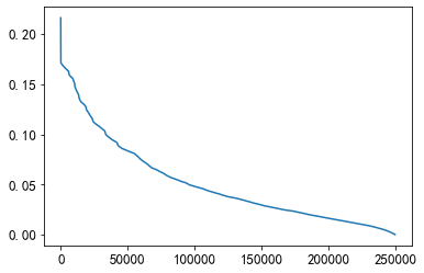

3.6.2. The average value of the creation time difference of articles clicked before and after

# 前后点击的文章的创建时间差的平均值
mean_diff_created_time = user_click_merge.groupby('user_id')['click_timestamp',
                         'created_at_ts'].apply(lambda x: mean_diff_time_func(x, 'created_at_ts'))

plt.plot(sorted(mean_diff_created_time.values, reverse=True))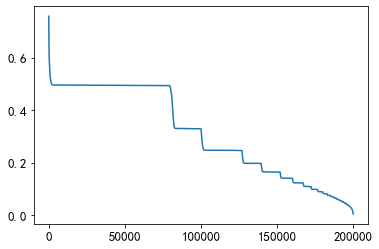

From the above figure, it can be found that the time difference between different users clicking on the article is different. Users click on the article successively, and the creation time of the article is also different.

4. Check the similarity list of articles before and after getting users

4.1. Word vectors for training news

from gensim.models import Word2Vec
import logging, pickle

# 需要注意这里模型只迭代了一次
def trian_item_word2vec(click_df, embed_size=16, save_name='item_w2v_emb.pkl', split_char=' '):
    #按click_timestamp排序
    click_df = click_df.sort_values('click_timestamp')
    
    # 将click_article_id转换成字符串才可以进行训练
    click_df['click_article_id'] = click_df['click_article_id'].astype(str)
    
    # 将click_article_id转换成句子的形式
    docs = click_df.groupby(['user_id'])['click_article_id'].apply(lambda x: list(x)).reset_index()
    docs = docs['click_article_id'].values.tolist()

    # 为了方便查看训练的进度，这里设定一个log信息
    logging.basicConfig(format='%(asctime)s:%(levelname)s:%(message)s', level=logging.INFO)

    # 这里的参数对训练得到的向量影响也很大,默认负采样为5
    w2v = Word2Vec(docs, vector_size=16, sg=1, window=5, seed=2020, workers=24, min_count=1, epochs=10)
    
    # 保存成字典的形式
    item_w2v_emb_dict = {k: w2v.wv[k] for k in click_df['click_article_id']}
    
    return item_w2v_emb_dict

item_w2v_emb_dict = trian_item_word2vec(user_click_merge)

4.2. Check the similarity of articles viewed by users before and after

# 随机选择5个用户，查看这些用户前后查看文章的相似性
sub_user_ids = np.random.choice(user_click_merge.user_id.unique(), size=15, replace=False)
sub_user_info = user_click_merge[user_click_merge['user_id'].isin(sub_user_ids)]# .isin（）筛选行

sub_user_info.head()

4.3. Check the similarity list of articles before and after getting users

# 得到用户前，后查看文章的相似度列表
def get_item_sim_list(df):
    sim_list = []
    item_list = df['click_article_id'].values
    for i in range(0, len(item_list)-1):
        emb1 = item_w2v_emb_dict[str(item_list[i])] # 需要注意的是word2vec训练时候使用的是str类型的数据
        emb2 = item_w2v_emb_dict[str(item_list[i+1])]
        sim_list.append(np.dot(emb1,emb2)/(np.linalg.norm(emb1)*(np.linalg.norm(emb2))))
    sim_list.append(0)
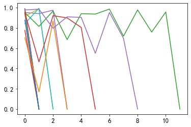
    return sim_list

4.4. View the similarity list of articles before and after visualizing users

for _, user_df in sub_user_info.groupby('user_id'):
    item_sim_list = get_item_sim_list(user_df)
    plt.plot(item_sim_list)

[Zero-Based Entry Recommendation System-News Recommendation] 1-Data Analysis-Tianchi Study Competition Notes

1. Data preprocessing

1.1. Calculate user click rank and number of clicks