1. Logistic regression algorithm
1. What is Logistic Regression
Logistic regression is such a process: facing a regression or classification problem, establish a cost function, then iteratively solve the optimal model parameters through optimization methods, and then test and verify the quality of our solved model.
Although Logistic regression has "regression" in its name, it is actually a classification method, mainly used for two-category problems (that is, there are only two types of output, representing two categories respectively)
In the regression model, y is a qualitative variable, such as y=0 or 1, and the logistic method is mainly used to study the probability of certain events
2. Advantages and disadvantages of logistic regression
advantage:
1) Fast, suitable for binary classification problems
2) Simple and easy to understand, directly see the weight of each feature
3) The model can be easily updated to absorb new data
shortcoming:
The ability to adapt to data and scenarios has limitations, and is not as adaptable as the decision tree algorithm
3. The difference between logistic regression and multiple linear regression
Logistic regression and multiple linear regression actually have many similarities. The biggest difference is that their dependent variables are different, and the others are basically the same. Because of this, the two regressions can be attributed to the same family, generalized linear models.
4. Logistic regression uses
Finding risk factors: looking for risk factors for a certain disease, etc.;
Prediction: According to the model, predict the probability of a certain disease or a certain situation under different independent variables;
Discrimination: In fact, it is somewhat similar to prediction. It is also based on the model to judge the probability that a person belongs to a certain disease or a certain situation, that is, to see how likely this person is to belong to a certain disease.
5. Regression general steps
Find the h function (i.e. the prediction function)
Construct J function (loss function)
Find a way to minimize the J function and find the regression parameters (θ)
6. Construct prediction function h(x)
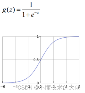
1) Logistic function (or called Sigmoid function), the function form is:
For the case of a linear boundary, the boundary form is as follows:
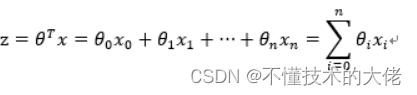
Among them, the training data is a vector
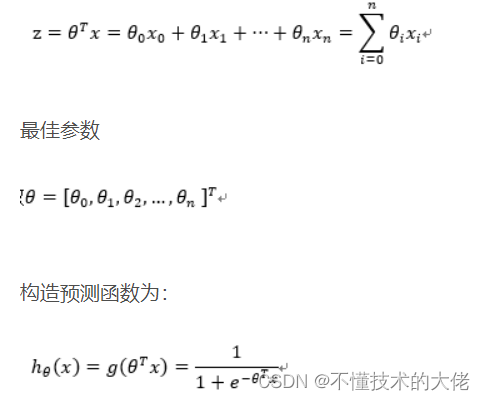
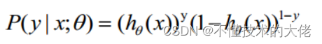
The value of the function h(x) has a special meaning, which represents the probability of the result being 1, so the probabilities of class 1 and class 0 for the input x are:
P(y=1│x;θ)=h_θ (x)
P(y=0│x;θ)=1-h_θ (x)
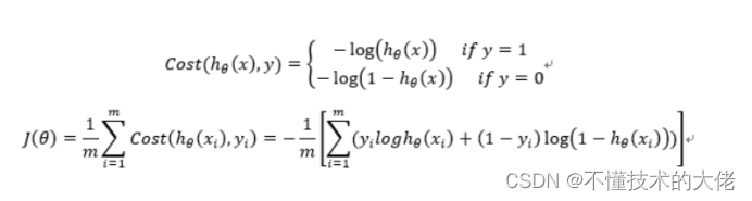
7. Construct loss function J (m samples, each sample has n features)
The Cost function and the J function are as follows, which are derived based on maximum likelihood estimation.
8. Detailed derivation process of loss function
1) The probability of the cost function
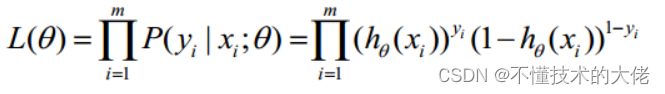
is combined and written as:
Take the likelihood function as:
The log-likelihood function is:

The maximum likelihood estimation is to find the θ when l(θ) takes the maximum value. In fact, the gradient ascent method can be used here to solve the problem. The obtained θ is the optimal parameter required.
In Andrew Ng's course, J(θ) is taken as the following formula, namely:

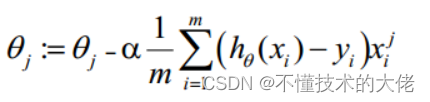
- Gradient descent method to find the minimum value
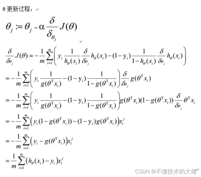
The θ update process can be written as:
9. Vectorization
Ectorization uses matrix calculations instead of for loops to simplify the calculation process and improve efficiency.
Vectorization process:
The matrix form of the agreed training data is as follows, each row of x is a training sample, and each column is a different special value:

The parameter A of g(A) is a column vector, so the implementation of the g function must support column vectors as parameters and return column vectors.
The θ update process can be changed to:

To sum up, the steps of θ update after Vectorization are as follows:
- Find A=x*θ
- E=g(A)-y

10. Regularization
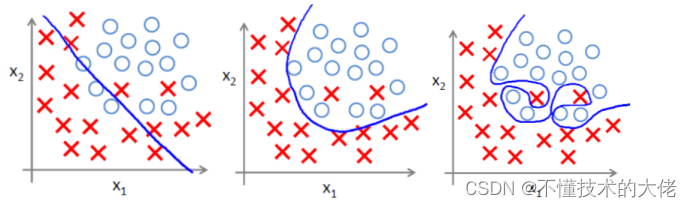
(1) Over-fitting problem
Over-fitting means over-fitting the training data, which increases the complexity of the model and makes it less prosperous (the ability to predict unknown data). The left picture
below is under-fitting, and the middle picture is Proper fit, overfitting on the right.
(2) The main reason for overfitting
Overfitting problems often arise from having too many features
Solution
1) Reduce the number of features (reducing features will lose some information, even if the features are well selected)
• Features to be retained can be manually selected;
• Model selection algorithm;
2) Regularization (more effective when there are many features)
• Preserve all features, but reduce the size of θ
(3) Regularization method
Regularization is the realization of the structural risk minimization strategy, which is to add a regularization item or penalty item to the empirical risk. The regularization term is generally a monotonically increasing function of the model complexity, the more complex the model, the larger the regularization term.
The regular term can take different forms. In the regression problem, the square loss is taken, which is the L2 norm of the parameter, and the L1 norm can also be taken. When taking the squared loss, the loss function of the model becomes:
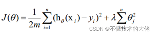
lambda is the regularization coefficient:
• If its value is large, it means that the complexity penalty for the model is large, and the loss penalty for the fitting data is small, so that it will not overfit the data, the deviation on the training data is large, and the loss penalty on the unknown data The variance is small, but underfitting may occur;
• If its value is small, it means that more attention is paid to fitting the training data, and the deviation on the training data will be small, but it may lead to overfitting.
The update of the regularized gradient descent algorithm θ becomes:

11. Python implements logistic regression:
from sklearn.linear_model import LogisticRegression
Model = LogisticRegression()
Model.fit(X_train, y_train)
Model.score(X_train,y_train)
# Equation coefficient and Intercept
Print(‘Coefficient’,model.coef_)
Print(‘Intercept’,model.intercept_)
# Predict Output
Predicted = Model.predict(x_test)
----- Part of the content is referenced from: Logistic Regression-Theory _pakko's Blog-CSDN Blog_Logistic Regression Binomial Distribution
2. K-means algorithm
1 Overview
K-means algorithm is the most classic partition-based clustering method and one of the top ten classic data mining algorithms. The basic idea of the K-means algorithm is to cluster the k points in the space and classify the objects closest to them. Through the iterative method, the value of each cluster center is updated successively until the best clustering result is obtained.
The k-means algorithm accepts the parameter k, and then divides the n data objects input in advance into k clusters so that the obtained clusters satisfy the similarity of objects in the same cluster, while objects in different clusters The similarity is small. The cluster similarity is calculated by using a "central object" (gravity center) obtained from the mean value of the objects in each cluster.
2. Implementation principle
The basic idea of the KMeans algorithm is to initially randomly set K cluster centers, and divide the sample points to be classified into each cluster according to the nearest neighbor principle. Then recalculate the centroids of each cluster according to the average method, so as to determine the new cluster center. Iterates until the moving distance of the cluster center is less than a given value.
The K-Means clustering algorithm is mainly divided into three steps:
(1) The first step is to find the cluster center for the points to be clustered;
(2) The second step is to calculate the distance from each point to the cluster center, and cluster each point into the nearest cluster to the point;
(3) The third step is to calculate the average value of the coordinates of all points in each cluster, and use this average value as the new cluster center;
Repeat (2) and (3) until the cluster center no longer moves in a large range or the number of clusters reaches the requirement.
The figure below shows the effect of K-means clustering on n sample points, where k is 2:
(a) Unclustered initial point set;
(b) Randomly select two points as cluster centers;
(c) Calculate the distance from each point to the cluster center, and cluster to the nearest cluster to the point;
(d) Calculate the mean value of the coordinates of all points in each cluster, and use this mean value as the new cluster center;
(e) Repeat (c), calculate the distance from each point to the cluster center, and cluster to the nearest cluster to the point;
(f) Repeat (d), calculate the average coordinates of all points in each cluster, and use this average as the new cluster center.
The biggest advantage of this algorithm is its simplicity and speed. The key of the algorithm lies in the selection of the initial center and the distance formula.
The value of K:
There is no optimal method to determine the number of clusters K, and it usually needs to be selected manually according to the specific problem. There is no direct cluster evaluation method for unsupervised clustering, but the effect of clustering can be evaluated from the degree of density within a cluster and the degree of dispersion between clusters. The most common methods are Silhouette Coefficient and Calinski-Harabaz Index. Among them, the calculation of Calinski-Harabaz Index is straightforward and simple, and the larger the result obtained, the better the clustering effect. Calculated as follows:
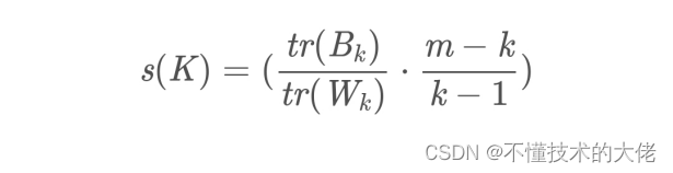
Among them: m is the number of samples in the training set, and k is the number of categories. Bk is the covariance matrix between categories, and Wk is the covariance matrix between internal data. tr is the trace of the matrix.
That is to say, the smaller the covariance of the internal data, the better, and the larger the covariance between categories, the better, so that the corresponding Calinski-Harabaz Index score will be higher. Main
steps:
Among the N data, randomly select K data ( That is, the final clustering is K class) as the initial center of clustering.
Calculate the Euclidean distance from each data point to the K center points separately, and assign it to the cluster which is closest to the center point.
Recalculate the coordinate mean of the K cluster data, and use the new mean as the center of the cluster.
Repeat steps 2 and 3 until the coordinates of the cluster centers are no longer transformed or the specified number of iterations is reached to form the final K clusters.
The k-Means algorithm, also known as k-means or k-means, is a widely used clustering algorithm or forms the basis of other clustering algorithms.
Assuming that the input sample is S=x.....m, the algorithm steps are:
select the initial k category centers μ2.Hk
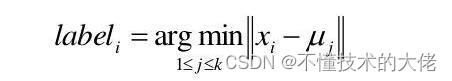
for each sample x;, and mark it as the category closest to the category center, namely:
Update each class center to be the mean of all samples belonging to that class

The last two steps are repeated until the variation of the class centers is less than some threshold.
Termination condition:
number of iterations) cluster center rate of change/minimum square error MSE (Minimum Squared Error)
Record K cluster centers as M,μ,,k, and the number of samples in each cluster as N,N2,..,N.
Use the squared error as the objective function:
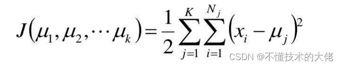
Find the partial derivative of the function with respect to from,...,Hp, its stagnation point is:

- Summary of k-Means clustering method
(1) Advantages:
It is a classic algorithm for solving clustering problems. It is simple and fast for processing large data sets. The algorithm maintains scalability and high efficiency. When the cluster is approximately Gaussian distributed, it The effect is better
(2) Disadvantage:
it can only be used when the average value of the cluster can be defined, it may not be suitable for some applications,
k (the number of clusters to be generated) must be given in advance, and it is sensitive to the initial value, Different initial values may lead to different results.
Not suitable for finding clusters with non-convex shapes or clusters with large differences in size. Sensitive to noise and outlier data,
but can be used as the basic algorithm for other clustering methods, such as spectral clustering. - Realize the code with JAVA:
class point { public float x = 0; public float y = 0; public int flage = -1; public float getX() { return x; } public void setX(float x) { this.x = x ; () { return y; } public void setY(float y) { this.y = y; } } public class Kcluster { point[] ypo;// point set point[] pacore = null;// old cluster center point [] pacoren = null;// new clustering center // preliminary clustering center, point set public void productpoint() { Scanner cina = new Scanner(System.in);
System.out.print("Please enter the number of points in the cluster (randomly generated):");
int num = cina.nextInt();
ypo = new point[num];
// Randomly generate points
for (int i = 0; i < num; i++) { float x = (int) (new Random().nextInt(10)); float y = (int) (new Random().nextInt(10)); ypo[i] = new point();// Object creation ypo[i].setX(x); ypo[i].setY(y); } // Initialize the cluster center position System.out.print("Please enter the initialization cluster The number of centers (randomly generated): "); int core = cina.nextInt(); this.pacore = new point[core];// store the cluster center this.pacoren = new point[core]; Random rand = new Random();
int temp[] = new int[core];
temp[0] = rand.nextInt(num);
pacore[0] = new point();
pacore[0].x = ypo[temp[0]].x;
pacore[0].y = ypo[temp[0]].y;
pacore[0].flage = 0;
// Avoid duplicate centers
for (int i = 1; i < core; i++) { int flage = 0; int thistemp = rand.nextInt(num); for (int j = 0; j < i; j++) { if (temp[j] == thistemp) { flage = 1;// has repeated break; } } if (flage == 1) { i--;
} else { pacore[i] = new point(); pacore[i].x = ypo[thistemp].x; pacore[i].y = ypo[thistemp].y; pacore[i].flage = 0; // 0 means cluster center } } System.out.println("Initial cluster center:"); for (int i = 0; i < pacore.length; i++) { System.out.println(pacore[i] .x + " " + pacore[i].y); } } // /// Find out which cluster center each point belongs to public void searchbelong()// Find out which cluster center each point belongs to { for (int i = 0; i < ypo.length; i++) { double dist = 999; int lable = -1;
for (int j = 0; j < pacore.length; j++) {
double distance = distpoint(ypo[i], pacore[j]);
if (distance < dist) {
dist = distance;
lable = j;
// po[i].flage = j + 1;// 1,2,3......
}
}
ypo[i].flage = lable + 1;
}
}
// 更新聚类中心
public void calaverage() {
for (int i = 0; i < pacore.length; i++) {
System.out.println("以<" + pacore[i].x + "," + pacore[i].y + ">为中心的点:");
int numc = 0;
point newcore = new point();
for (int j = 0; j < ypo.length; j++) { if (ypo[j].flage == (i + 1)) { System.out.println(ypo[j].x + "," + ypo[j].y); numc += 1; newcore.x += ypo[j].x; newcore.y += ypo[j].y; } } // new cluster center (that is, all aggregation The center of the point) pacoren[i] = new point(); pacoren[i].x = newcore.x / numc;//sum of x coordinates of all clustering elements/number of elements pacoren[i].y = newcore.y / numc; pacoren[i].flage = 0; System.out.println("New cluster center: " + pacoren[i].x + "," + pacoren[i].y); } }
public double distpoint(point px, point py) { return Math.sqrt(Math.pow((px.x - py.x), 2) + Math.pow((px.y - py.y), 2)) ; } public void change_oldtonew(point[] old, point[] news) { for (int i = 0; i < old.length; i++) { old[i].x = news[i].x; old[i ].y = news[i].y; old[i].flage = 0;//Represented as the flag of the cluster center. } } public void movecore() { // this.productpoint();//initialization, sample set, cluster center, this.searchbelong(); this.calaverage();// double moveddistance = 0; int biao = - 1;// sign, whether the movement of the cluster center point meets the minimum distance
for (int i = 0; i < pacore.length; i++) { moveddistance = distpoint(pacore[i], pacoren[i]);//Calculate the distance between the new and old center points System.out.println("distcore: " + moveddistance);// The moving distance of the cluster center if (movedistance < 0.01) { biao = 0; } else { biao = 0; } else { biao = 1;// Continue to iterate, break; } } if ( biao == 0) { System.out.print("iteration complete!!!!"); } else { change_oldtonew(pacore, pacoren); movecore(); } }
public static void main(String[] args) {
// TODO Auto-generated method stub
Kcluster kmean = new Kcluster();
kmean.productpoint();
kmean.movecore();
}
}
----Part of the content is referenced from: https://blog.csdn.net/weixin_40479663/article/details/82974625?utm_source=app&app_version=4.10.0&code=app_1562916241&uLinkId=usr1mkqgl919blen